<?xml version="1.0" encoding="utf-8"?><feed xmlns="http://www.w3.org/2005/Atom" ><generator uri="https://jekyllrb.com/" version="3.10.0">Jekyll</generator><link href="https://jan-a-krzywda.github.io/feed.xml" rel="self" type="application/atom+xml" /><link href="https://jan-a-krzywda.github.io/" rel="alternate" type="text/html" /><updated>2026-08-01T07:18:36+02:00</updated><id>https://jan-a-krzywda.github.io/feed.xml</id><title type="html">Jan A. Krzywda</title><subtitle>Personal site and blog.</subtitle><author><name>Jan A. Krzywda</name></author><entry><title type="html">Bypassing the Latency Bottleneck: On-Chip Logic for Real-Time Shadow Tomography</title><link href="https://jan-a-krzywda.github.io/2026/05/bypassing-the-latency-bottleneck-on-chip-logic-for-real-time-shadow-tomography/" rel="alternate" type="text/html" title="Bypassing the Latency Bottleneck: On-Chip Logic for Real-Time Shadow Tomography" /><published>2026-05-18T13:27:10+02:00</published><updated>2026-05-18T13:27:10+02:00</updated><id>https://jan-a-krzywda.github.io/2026/05/bypassing-the-latency-bottleneck-on-chip-logic-for-real-time-shadow-tomography</id><content type="html" xml:base="https://jan-a-krzywda.github.io/2026/05/bypassing-the-latency-bottleneck-on-chip-logic-for-real-time-shadow-tomography/"><![CDATA[<p><a class="github-badge" href="https://github.com/jan-a-krzywda/quantum-gym/tree/main/shadow_gym"><img src="/assets/images/25231.png" alt="" class="github-logo" /> GitHub Repo</a></p>

<p>Environments with many constrains often drive most relevant leaps. The same holds true for near-term quantum hardware, including <a href="https://www.quantum-inspire.com/">Quantum Inspire</a> device.</p>

<h4 id="tldr">TL;DR</h4>

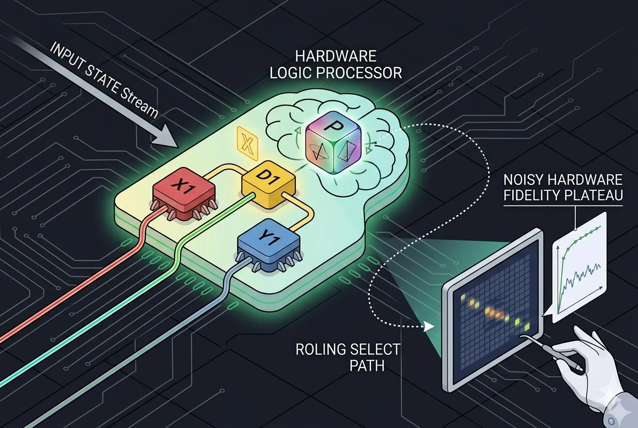
<p>Recently, driven by a requirement to quickly characterize a quantum state on a real hardware, I attempted to implement a shadow tomography protocol on the Quantum Inspire platform. However, I quickly faced a severe hardware bottleneck: it lacked support for the parameterized circuits needed for shot-by-shot sampled Pauli measurements. I was forced to choose between running the exact same circuit for thousands of shots (yielding poor tomographic data) or running thousands of different circuits in separate jobs (suffering from crippling queue and network latencies). Then, I thought about a third way: I designed a protocol for shadow tomography that bypasses the classical-quantum bottleneck entirely by embedding the classical decision process directly into the quantum circuit.</p>

<figure class="post-figure">
  <img src="/assets/images/latency1.webp" alt="" loading="lazy" />
</figure>

<h4 id="the-measure-first-paradigm">The Measure-First Paradigm</h4>

<p>Finding classical representations of a quantum state in polynomial time has completely changed how we approach quantum information processing (Aaronson <a href="https://arxiv.org/abs/1711.01053">arXiv:1711.01053</a>). Shadow-based algorithms have implemented a “measure first, ask questions later” paradigm, effectively treating the quantum computer as a feature processor that generates data for instance for a classical machine learning model.</p>

<p>The most common realization of this paradigm is shadow tomography via random Pauli measurements (Huang <a href="https://arxiv.org/abs/2002.08953">arXiv:2002.08953</a>). Theoretically, it is elegant and straightforward: apply a random single-qubit rotation, then read out in the computational basis. In practice, however, this requires a uniquely randomized circuit for every single shot. On many cloud-based platforms, this constant classical-to-quantum ping-pong introduces massive latency.</p>

<p>To overcome this, we need a protocol compatible with any platform that supports quantum non-demolition (QND) mid-circuit measurements.</p>

<h4 id="the-on-chip-logic">The On-Chip Logic</h4>

<p>The key idea is to use a mid-circuit measurement to collapse a set of ancilla qubits into a random basis choice, which is then used to control the measurement basis of the data qubits. This allows us to effectively implement a random measurement process natively on the chip, without waiting for a classical compiler.</p>

<p>The protocol operates in six steps:</p>

<ol>
  <li><strong>Prepare</strong> the data qubits in the state of interest.</li>
  <li><strong>Initialize</strong> a set of ancilla qubits in a superposition state that encodes the desired probability distribution over the measurement bases.</li>
  <li><strong>Measure</strong> the ancillas mid-circuit, collapsing them into a specific basis choice.</li>
  <li><strong>Feed-forward</strong> the measurement outcome to control the application of single-qubit rotations on the data qubits, physically altering the measurement basis for that specific shot.</li>
  <li><strong>Readout</strong> the data qubits in the standard computational basis.</li>
  <li><strong>Reconstruct</strong> the classical shadow by feeding the collected data into a classical algorithm to estimate the quantum state.</li>
</ol>

<h4 id="the-hardware-gadget">The Hardware Gadget</h4>

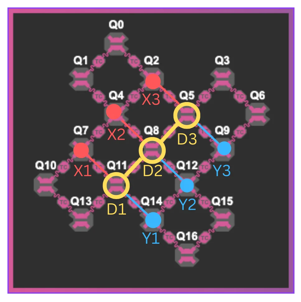
<p>The core of this protocol relies on a specific “gadget”: one data qubit paired with two dedicated ancilla qubits. If our data qubits are kept in a line, this amounts to a tri-linear connectivity pattern where each data qubit is directly connected to two ancillas. As a proof of principle, we concentrate on a 3-qubit cluster state, which requires 3 data qubits and 6 ancillas in total.</p>

<figure class="post-figure">
  <img src="/assets/images/latency2.webp" alt="Hardware Topology: A 3-qubit cluster state implementation mapped onto the chip. The central data qubits (yellow, D1–D3) are each coupled to two dedicated &quot;dice&quot; ancilla qubits—one for controlling the X-basis (red, X1–X3) and one for the…" loading="lazy" />
  <figcaption><strong>Hardware Topology:</strong> A 3-qubit cluster state implementation mapped onto the chip. The central data qubits (yellow, D1–D3) are each coupled to two dedicated "dice" ancilla qubits—one for controlling the X-basis (red, X1–X3) and one for the Y-basis (blue, Y1–Y3)—forming the required tri-linear connectivity pattern.</figcaption>
</figure>

<p>The two ancillas act as our classical dice. One ancilla controls the X vs. Z basis choice via a controlled-R_y(-\pi/2) rotation. The second ancilla controls the Y vs. Z basis choice via a controlled-R_x(\pi/2) rotation.</p>

<table>
  <tbody>
    <tr>
      <td>If we initialize the ancillas in the</td>
      <td>+&gt; state, they yield a uniform distribution over the outcomes. Because the controlled rotations apply based on these outcomes, the data qubit’s measurement basis maps out as follows.</td>
    </tr>
  </tbody>
</table>

<ul>
  <li><strong>00</strong> - Z basis (no rotation), 25% probability.</li>
  <li><strong>10</strong> - X basis (via Ry(-\pi/2)), 25% probability.</li>
  <li><strong>01</strong> - Y basis (via Rx(\pi/2)), 25% probability.</li>
  <li><strong>11</strong> - Y basis (via Ry(-\pi/2) followed by R_x(\pi/2)), 25% probability.</li>
</ul>

<table>
  <tbody>
    <tr>
      <td>Notice a slight collision? Due to the non-commuting nature of the rotations, the 11 outcome also results in a Y-basis measurement. This means a naive</td>
      <td>+&gt; initialization actually measures Y 50% of the time!</td>
    </tr>
  </tbody>
</table>

<p>To account for this, we can easily correct the bias by adjusting the initial rotation angles of the ancillas. We map our desired target probabilities px, py, pz into precise physical rotation angles theta1 and theta2:</p>

<div class="language-plaintext highlighter-rouge"><div class="highlight"><pre class="highlight"><code>def softmax_to_angles(px: float, py: float, pz: float) -&gt; Tuple[float, float]:
    p2 = py
    p1 = px / (px + pz + 1e-12)

    theta1 = 2.0 * np.arcsin(np.sqrt(np.clip(p1, 0, 1)))
    theta2 = 2.0 * np.arcsin(np.sqrt(np.clip(p2, 0, 1)))
    return theta1, theta2
</code></pre></div></div>

<p>We then apply these angles to the ancillas during the initialization step:</p>

<div class="language-plaintext highlighter-rouge"><div class="highlight"><pre class="highlight"><code>for i, dq in enumerate(DATA_QUBITS):
        a1, a2 = ANCILLA_MAP[dq]
        if theta1_per_qubit[i] != 0:
            qc.ry(theta1_per_qubit[i], a1)
        if theta2_per_qubit[i] != 0:
            qc.ry(theta2_per_qubit[i], a2)
    qc.barrier()
</code></pre></div></div>

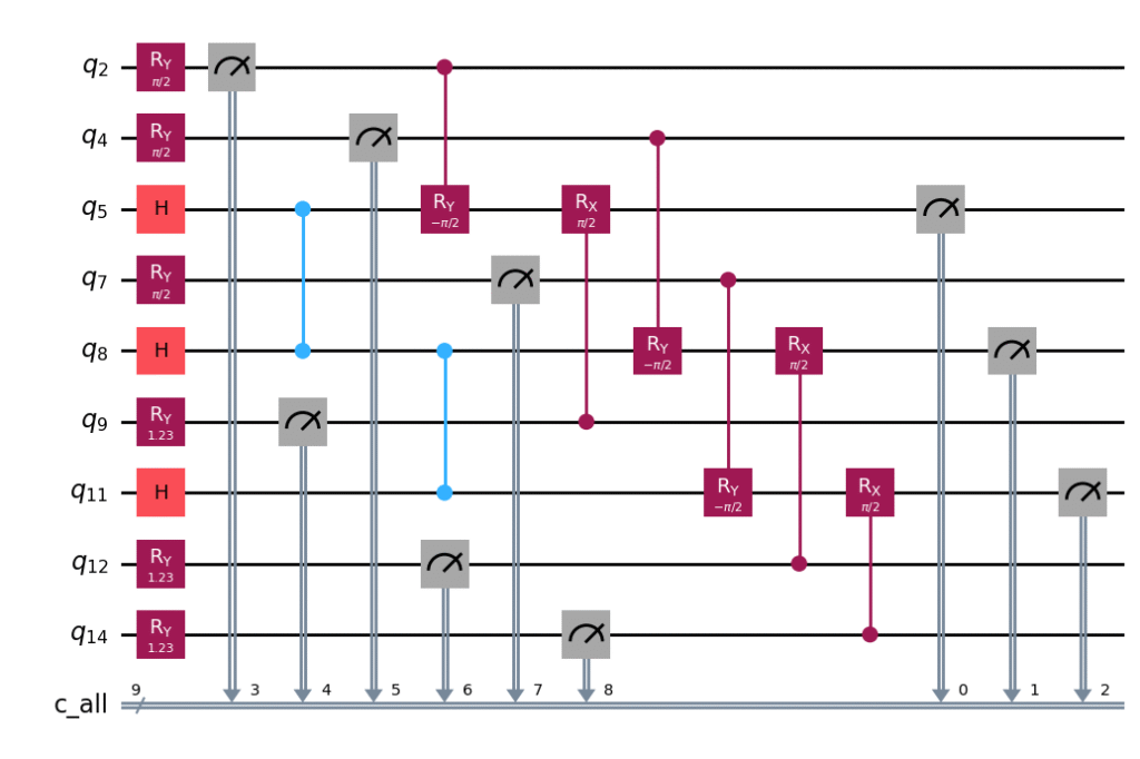
<p>As showed in the circuit below, to get a uniform distribution px = py = pz = 1/3, we need theta1 and theta2 ~ 70.5 deg.</p>

<figure class="post-figure">
  <img src="/assets/images/image-10-1024x682.png" alt="The &quot;Hardware Softmax&quot; Circuit: The physical circuit implementation of the on-chip logic protocol. A 3-qubit cluster state is prepared on the central data qubits (q_5, q_8, q_{11}). The six dedicated ancilla qubits are initialized with…" loading="lazy" />
  <figcaption><strong>The "Hardware Softmax" Circuit:</strong> The physical circuit implementation of the on-chip logic protocol. A 3-qubit cluster state is prepared on the central data qubits (q_5, q_8, q_{11}). The six dedicated ancilla qubits are initialized with specific rotation angles (e.g., 1.23 rad ~ 70.5 deg) to encode the desired uniform measurement distribution. Mid-circuit measurements on these ancillas are then used to dynamically control the R_y(-\pi/2) and R_x(\pi/2) basis-change operations on the data qubits, natively executing the randomized shadow sampling right before the final readout.</figcaption>
</figure>

<h3 id="results">Results</h3>

<table>
  <tbody>
    <tr>
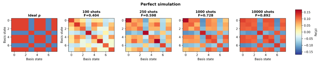
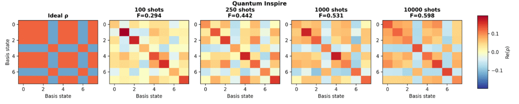
      <td>To validate the protocol, I ran this shadow tomography procedure on Quantum Inspire to characterize a 3-qubit cluster state, which has three stabilizers K_i</td>
      <td>psi&gt; = c_i</td>
      <td>psi&gt;. As you can see in the density matrix heatmaps below, qualitatively, the reconstructed density matrix matches the ideal state, proving that the mid-circuit logic executes the randomized measurements.</td>
    </tr>
  </tbody>
</table>

<figure class="post-figure">
  <img src="/assets/images/image-5-1024x205.png" alt="Ideal Simulation: Real parts of the reconstructed density matrices from a perfect, noise-free simulation of the hardware-logic protocol. As the shot count scales, the reconstructed matrix rapidly and accurately converges to the ideal…" loading="lazy" />
  <figcaption><strong>Ideal Simulation:</strong> Real parts of the reconstructed density matrices from a perfect, noise-free simulation of the hardware-logic protocol. As the shot count scales, the reconstructed matrix rapidly and accurately converges to the ideal 3-qubit cluster state.</figcaption>
</figure>
<figure class="post-figure">
  <img src="/assets/images/image-8-1024x205.png" alt="Hardware Reconstruction: Real parts of the density matrices reconstructed natively on the Quantum Inspire hardware. While the structural footprint qualitatively matches the ideal state perfectly, hardware noise heavily dampens the…" loading="lazy" />
  <figcaption><strong>Hardware Reconstruction:</strong> Real parts of the density matrices reconstructed natively on the Quantum Inspire hardware. While the structural footprint qualitatively matches the ideal state perfectly, hardware noise heavily dampens the amplitudes of the off-diagonal elements.</figcaption>
</figure>

<p>However, the reduced amplitudes of the off-diagonal density matrix elements suggest the presence of imperfections, which are most likely dominated by the limited fidelity of the gates and mid-circuit measurements on the hardware.</p>

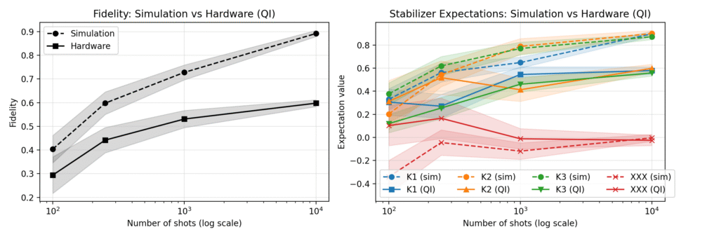
<p>This is confirmed when we look at the fidelity between the target state and the reconstructed one, as well as the reconstructed stabilizer expectation values, which are all significantly reduced from the ideal value of 1. For comparison, we also plotted an observable that is expected to be zero.</p>

<figure class="post-figure">
  <img src="/assets/images/image-9-1024x341.png" alt="Convergence Metrics: (Left) State fidelity scaling with the number of shots. (Right) Convergence of the reconstructed stabilizer expectation values (K_1, K_2, K_3) and a baseline observable expected to be zero (XXX). The gap between the…" loading="lazy" />
  <figcaption><strong>Convergence Metrics:</strong> <em>(Left)</em> State fidelity scaling with the number of shots. <em>(Right)</em> Convergence of the reconstructed stabilizer expectation values (K_1, K_2, K_3) and a baseline observable expected to be zero (XXX). The gap between the simulation (dashed lines) and hardware (solid lines) highlights the plateauing effect caused by gate and mid-circuit measurement infidelities on physical chips.</figcaption>
</figure>

<h3 id="next-steps">Next steps</h3>

<p>While this demonstration utilized a uniform distribution over the three Pauli bases, the true power of this “Hardware Logic” lies in its tunability. In particular, I am planning to use the protocol to implement a more active learning-based shadow tomography, where the measurement distribution is adaptively updated based on the data collected in previous shots. While it cannot achieve the same level of universality as the original classical shadow protocol, I believe it can be significantly more powerful in the presence of noisy, biased, and limited data—which is the reality of near-term quantum hardware.</p>]]></content><author><name>Jan A. Krzywda</name></author><category term="code" /><summary type="html"><![CDATA[Environments with many constrains often drive most relevant leaps. The same holds true for near-term quantum hardware, including the Quantum Inspire device.]]></summary><media:thumbnail xmlns:media="http://search.yahoo.com/mrss/" url="https://jan-a-krzywda.github.io/assets/images/latency1.webp" /><media:content medium="image" url="https://jan-a-krzywda.github.io/assets/images/latency1.webp" xmlns:media="http://search.yahoo.com/mrss/" /></entry><entry><title type="html">Erratiq: Human Perception for Quantum Error Decoding</title><link href="https://jan-a-krzywda.github.io/2026/04/erratiq-human-perception-for-quantum-error-decoding/" rel="alternate" type="text/html" title="Erratiq: Human Perception for Quantum Error Decoding" /><published>2026-04-23T22:35:41+02:00</published><updated>2026-04-23T22:35:41+02:00</updated><id>https://jan-a-krzywda.github.io/2026/04/erratiq-human-perception-for-quantum-error-decoding</id><content type="html" xml:base="https://jan-a-krzywda.github.io/2026/04/erratiq-human-perception-for-quantum-error-decoding/"><![CDATA[<p><a href="https://erratiq.xyz/">Play the game</a></p>

<p><strong>TL;DR:</strong> You can help develop better quantum decoders by playing the <a href="https://erratiq.xyz/">Erratiq</a> game.</p>

<figure class="post-figure">
  <img src="/assets/images/image-7-1024x818.png" alt="Game startscreen" loading="lazy" />
  <figcaption>Game startscreen</figcaption>
</figure>

<p>Human perception allows us to automatically detect patterns. This evolutionary trait has been crucial for our survival, enabling us to recognize faces, navigate environments, and make sense of complex data. For centuries, detecting repeatable patterns and understanding the actions needed to affect them has been the cornerstone not only of survival, but of scientific discovery and technological advancement. Think of the citizen scientists in the <em>Foldit</em> project, whose spatial reasoning and human intuition allowed them to solve complex protein-folding structures that had stumped automated algorithms for years. What if we could employ this exact same ability to improve the performance of quantum error correction?</p>

<p>In principle, quantum error correction allows us to sustain meaningful computation on a quantum computer well beyond the physical limits imposed by the environment. It effectively stabilizes the fragile quantum state. When combined with fault-tolerant operations, it can unlock the full potential of quantum computing—bringing significant implications for cryptography, optimization, chemistry, and the simulation of complex quantum systems. This stabilization is made possible by building a certain redundancy into the encoding of quantum information, which allows us to detect and correct (or at least track) physical errors.</p>

<div class="fig-row">
<div class="fig-col">
<figure class="post-figure">
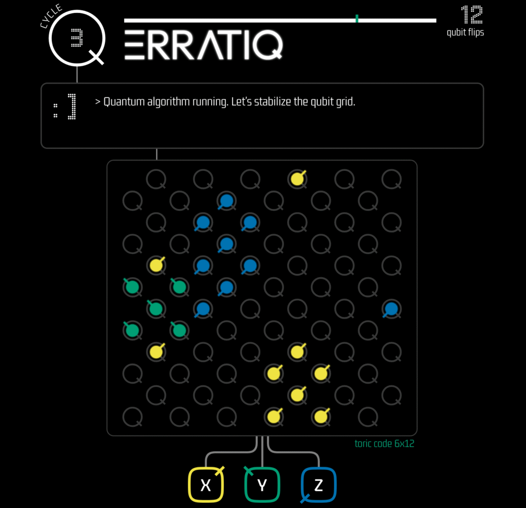
  <img src="/assets/images/image-8-1024x990.png" alt="Screen from the torric code (before correction). We use human-friendly representation to show stabilizer violations." loading="lazy" />
  <figcaption>Screen from the torric code (before correction). We use human-friendly representation to show stabilizer violations.</figcaption>
</figure>
</div>

<div class="fig-col">
<figure class="post-figure">
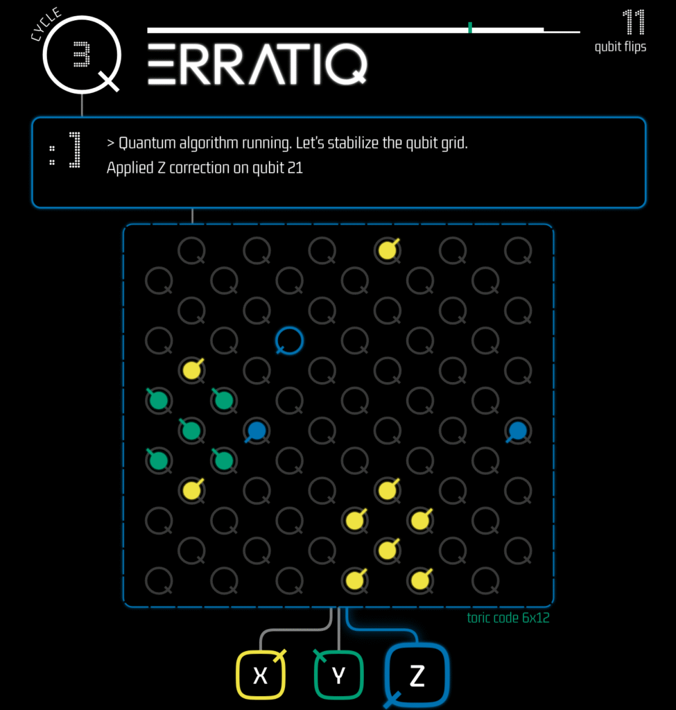
  <img src="/assets/images/image-11-975x1024.png" alt="Screen from the game (after correction)" loading="lazy" />
  <figcaption>Screen from the game (after correction)</figcaption>
</figure>
</div>
</div>

<p>However, none of this works without a <em>decoder</em>—a classical algorithm that converts the information from the sensors (syndromes) into a correction operation. While many decoders have been proposed, including minimum weight perfect matching, belief propagation, and machine learning-based approaches, they often struggle with scalability and real-time performance, especially as the size of quantum systems increases.</p>

<p>Recently, machine learning (ML) based decoders have shown immense promise. But they often require massive amounts of training data and computational resources, which can limit their practicality. For instance, a reinforcement learning (RL) agent starts with no prior knowledge of the system and must learn to make decisions solely based on feedback from its environment. As an illustrative example, consider an RL agent trained to decode a surface code of distance-15. The action space of the agent is astronomical, preventing any meaningful training without significant simplifications. And even with a simplified action space, the agent requires a massive number of training episodes to learn an effective decoding strategy, which is exceptionally time-consuming and computationally expensive.</p>

<p><strong>Why not ask a human for help?</strong></p>

<p>That is the idea behind <strong>Erratiq</strong>, a game designed in collaboration between Leiden University and <a href="https://www.waag.org/en/">Waag Futurelab</a> to harvest the potential of the human mind to guide the training of ML-based decoders for quantum error correction. By engaging players in a fun and interactive way, Erratiq aims to collect valuable data on how humans approach the problem of decoding quantum errors. This data can then be used to train more efficient and effective machine learning models.</p>

<p>The game is built to be accessible to a wide audience, regardless of their background in quantum computing, providing a platform for players to directly contribute to the advancement of quantum error correction research. In its first version, it already features a 72-qubit toric code and a 30-qubit LDPC code. The latter, in particular, represents a family of resource-efficient but hard-to-decode quantum error-correcting codes, making it an ideal candidate for testing how well human intuition can guide ML training.</p>

<figure class="post-figure">
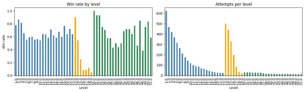
  <img src="/assets/images/image-9-1024x310.png" alt="Win rate and attempts in three codes: toric (blue), bicycle (yellow) and surface (green). The number of errors progresses with each level, and the players inherit number of flips." loading="lazy" />
  <figcaption>Win rate and attempts in three codes: toric (blue), bicycle (yellow) and surface (green). The number of errors progresses with each level, and the players inherit number of flips.</figcaption>
</figure>

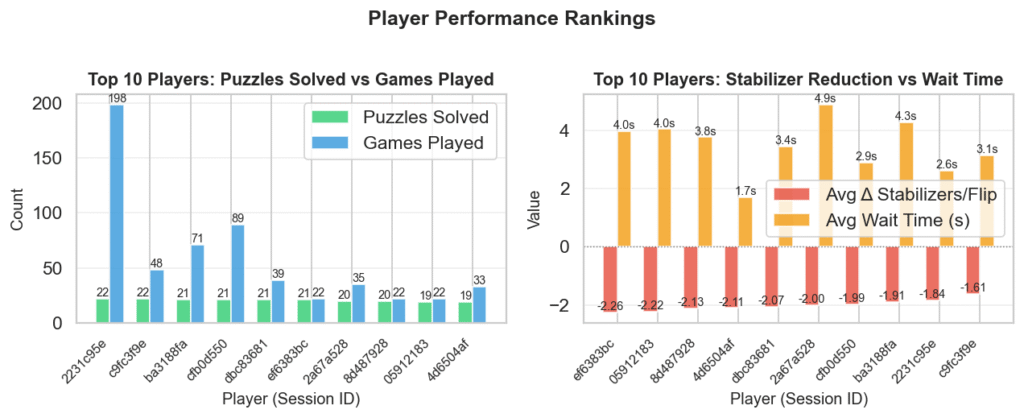
<p>So far, we have analyzed about 5,500 games and found that some players can already decode errors at a level comparable to state-of-the-art machine learning decoders, achieving a reduction in stabilizers per flip to below 2. However, to truly train a robust machine learning model, we need to collect a massive amount of data, and we are still in the early stages of this process.</p>

<figure class="post-figure">
  <img src="/assets/images/image-10-1024x418.png" alt="Top 10 players (23.04.2026) on the toric code levels." loading="lazy" />
  <figcaption>Top 10 players (23.04.2026) on the toric code levels.</figcaption>
</figure>

<p>This is where we need your help! By playing Erratiq, you can contribute to the advancement of quantum error correction research and help us unlock the full potential of quantum computing. Whether you are a seasoned gamer or just looking for a fun way to contribute to science, Erratiq offers an engaging and rewarding experience. So why not give it a try and see how your intuition can help shape the future of quantum computing?</p>

<p><strong>What will we do next?</strong> The dataset we collect will serve two main purposes:</p>

<ol>
  <li>As a prior for a reinforcement-learning agent, seeding the policy search with human-derived trajectories.</li>
  <li>As a training corpus for a decision-transformer model that will replicate human move sequences and produce an interpretable account of human decoding strategies.</li>
</ol>

<p>Next time, I will dive into the idea behind the decision transformer and show exactly how it can be used to train a machine learning model that replicates human decoding strategies for quantum error correction.</p>

<p><a href="https://erratiq.xyz/">Play the game</a></p>]]></content><author><name>Jan A. Krzywda</name></author><category term="code" /><summary type="html"><![CDATA[Human perception allows us to automatically detect patterns.]]></summary><media:thumbnail xmlns:media="http://search.yahoo.com/mrss/" url="https://jan-a-krzywda.github.io/assets/images/image-11-e1776976532677.png" /><media:content medium="image" url="https://jan-a-krzywda.github.io/assets/images/image-11-e1776976532677.png" xmlns:media="http://search.yahoo.com/mrss/" /></entry><entry><title type="html">Quantum Digital Twin: How I Trained AI to Hallucinate the Physics of a 17-Qubit Processor</title><link href="https://jan-a-krzywda.github.io/2026/04/quantum-digital-twin-how-i-trained-ai-to-hallucinate-the-physics-of-a-17-qubit-processor/" rel="alternate" type="text/html" title="Quantum Digital Twin: How I Trained AI to Hallucinate the Physics of a 17-Qubit Processor" /><published>2026-04-14T14:29:52+02:00</published><updated>2026-04-14T14:29:52+02:00</updated><id>https://jan-a-krzywda.github.io/2026/04/quantum-digital-twin-how-i-trained-ai-to-hallucinate-the-physics-of-a-17-qubit-processor</id><content type="html" xml:base="https://jan-a-krzywda.github.io/2026/04/quantum-digital-twin-how-i-trained-ai-to-hallucinate-the-physics-of-a-17-qubit-processor/"><![CDATA[<p><a class="github-badge" href="https://github.com/jan-a-krzywda/quantum-gym"><img src="/assets/images/25231.png" alt="" class="github-logo" /> GitHub Repo</a></p>

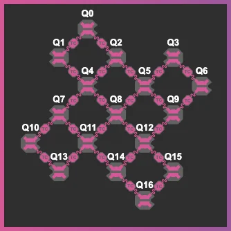
<p>I recently got my hands on a 17-qubit superconducting transmon device of Quantum Inspire (<a href="https://www.quantum-inspire.com/">https://www.quantum-inspire.com/</a>).</p>

<p>Before developing complex quantum algorithms, I wanted to build a systems-level understanding of the hardware. In particular, I wanted to understand the role of time and space in the noise, and how the qubits interact with each other as one complex system.</p>

<div class="fig-row">
<div class="fig-col" style="flex-basis:33.33%">
<figure class="post-figure">
  <img src="/assets/images/digital_twin1.webp" alt="Topography of the transmon device" loading="lazy" />
  <figcaption>Topography of the transmon device</figcaption>
</figure>
</div>

<div class="fig-col" style="flex-basis:66.66%">
<figure class="post-figure">
  <img src="/assets/images/image-6.png" alt="Device used in this blogpost" loading="lazy" />
  <figcaption>Device used in this blogpost</figcaption>
</figure>
</div>
</div>

<p>Initially, I explored standard quantum benchmarks and system identification methods, but neither approach provided the right level of insight. Metrics like T1​, T2​, Randomized Benchmarking (RB), and Gate Set Tomography (GST) provide detailed information on individual qubits and gates, but they often treat these components in isolation. Conversely, global benchmarks like Quantum Volume or CLOPS are time-averaged, boiling performance down to a few numbers. This abstraction can obscure the underlying physics and make it difficult to diagnose specific bottlenecks.</p>

<p>I was looking for a “middle ground”. a model that is both interpretable and holistic, capturing how these subsystems (qubits) actually behave and interact as a cohesive whole. In the long term, an effective model that accurately captures the system’s response can be used to train control policies and develop new, noise-resilient algorithms (akin to the concept of world models []).</p>

<p>Therefore, instead of relying on traditional physical modeling, I turned to unsupervised machine learning. Using a 1D Convolutional Variational Autoencoder (Conv-VAE), I constructed a data-driven, low-dimensional representation of a noisy 17-qubit processor, serving as a digital twin to generate artificial data.</p>

<div class="fig-row">
<div class="fig-col">
<figure class="post-figure">
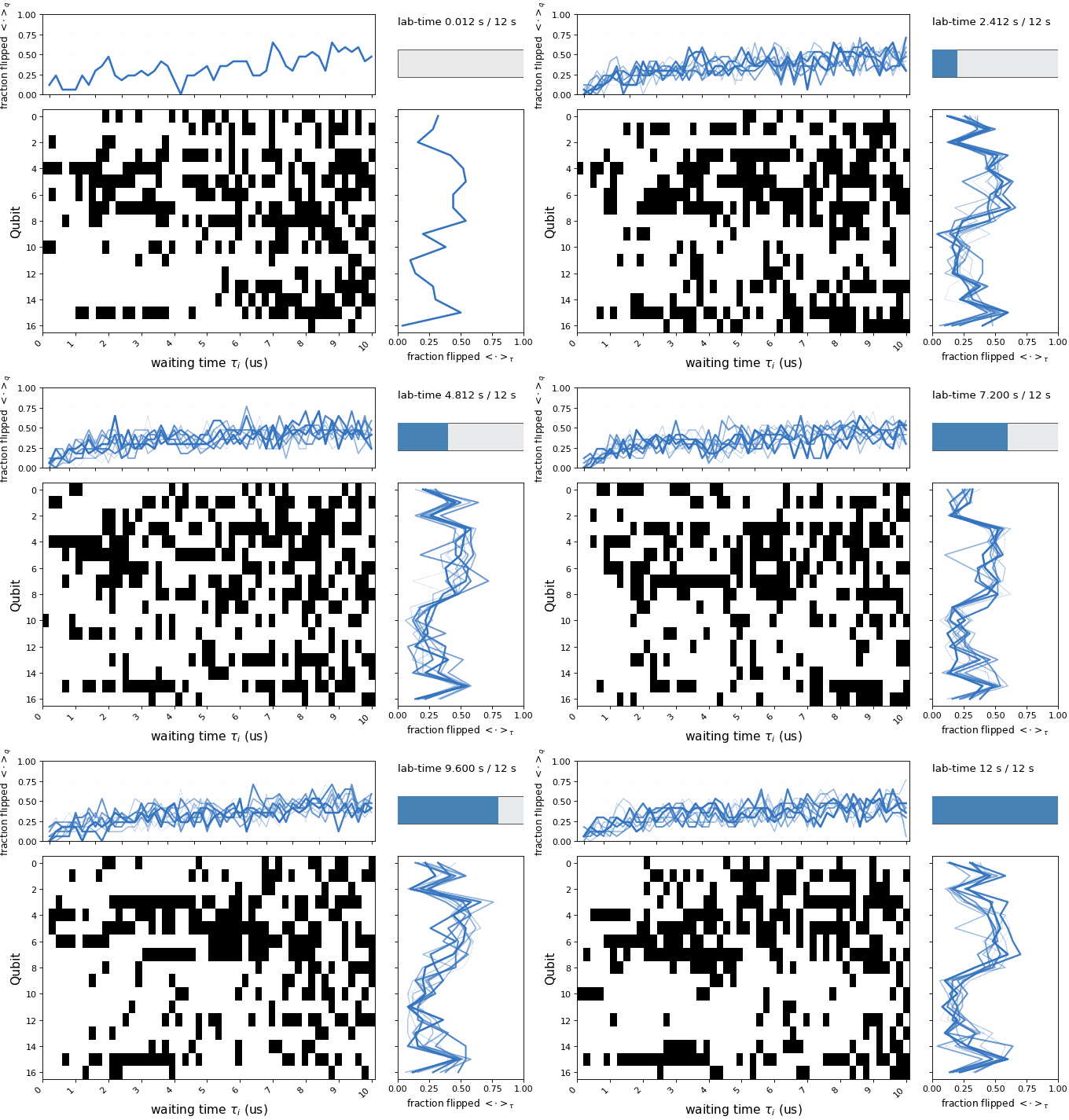
  <img src="/assets/images/fid_memory_3d_repetitions_2d_bin100.gif" alt="Signal from the real device. Return probability of superposition state at variable waiting time tau_i, averaged over 100 repetitions. 5000 repetitions in total (around 1 min)" loading="lazy" />
  <figcaption><strong>Signal from the real device.</strong> Return probability of superposition state at variable waiting time tau_i, averaged over 100 repetitions. 5000 repetitions in total (around 1 min)</figcaption>
</figure>
</div>

<div class="fig-col">
<figure class="post-figure">
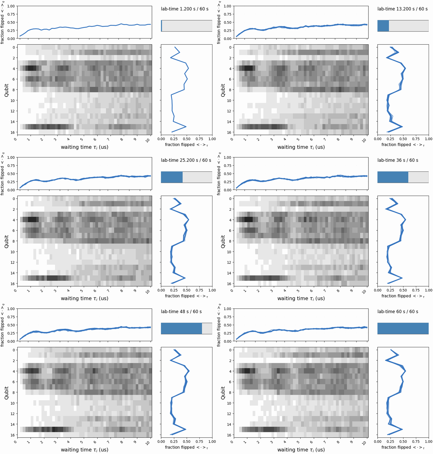
  <img src="/assets/images/vae_zebra_memory_3d_repetitions_2d_bin100-2.gif" alt="Artificial signal. The same signal, but from the digital twin (see below)" loading="lazy" />
  <figcaption><strong>Artificial signal. </strong>The same signal, but from the digital twin (see below)</figcaption>
</figure>
</div>
</div>

<p>Here is how I bypassed the standard formulas and let the data describe the hardware itself.</p>

<h2 id="1-the-probing-circuit-catching-the-hardware-in-the-act">1. The Probing Circuit (Catching the Hardware in the Act)</h2>

<p><strong>Revised Text</strong></p>

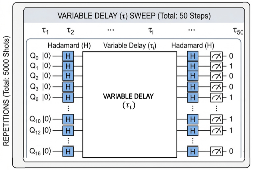
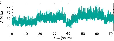
<p>To build a digital twin, I first needed a system fingerprint, a rich dataset mapping the chip across space and time. For starters, I decided to investigate the dephasing processes, which typically limit the achievable length of quantum circuits. I went with a simple probing circuit: H−delay(τ)−H applied simultaneously across all qubits for different waiting times τ. In the absence of noise, it should always return 0, but in reality, it did not.</p>

<p>I designed this sequence to be sensitive to both T1​ and T2* decay, as well as qubit-to-qubit correlations and spatiotemporal drift. To capture the latter, I swept the delay τ from 0.1 µs to 10 µs. This yields a single snapshot of the hardware’s behavior across all qubits. Next, this snapshot was repeated 5,000 times to observe exactly how the hardware slowly drifts. The probing sequence looks like this:</p>

<figure class="post-figure">
  <img src="/assets/images/scheme_twin-1.png" alt="The probing sequence: Simultaneously across all qubits, I performed a Free Induction Decay (FID) sequence with a variable waiting time, τi​. I swept τi​ across a range of waiting times, and this entire sweep was then repeated 5,000 times." loading="lazy" />
  <figcaption><strong>The probing sequence:</strong> Simultaneously across all qubits, I performed a Free Induction Decay (FID) sequence with a variable waiting time, τi​. I swept τi​ across a range of waiting times, and this entire sweep was then repeated 5,000 times.</figcaption>
</figure>

<h2 id="2-the-raw-hardware-fingerprint">2. The raw hardware fingerprint</h2>

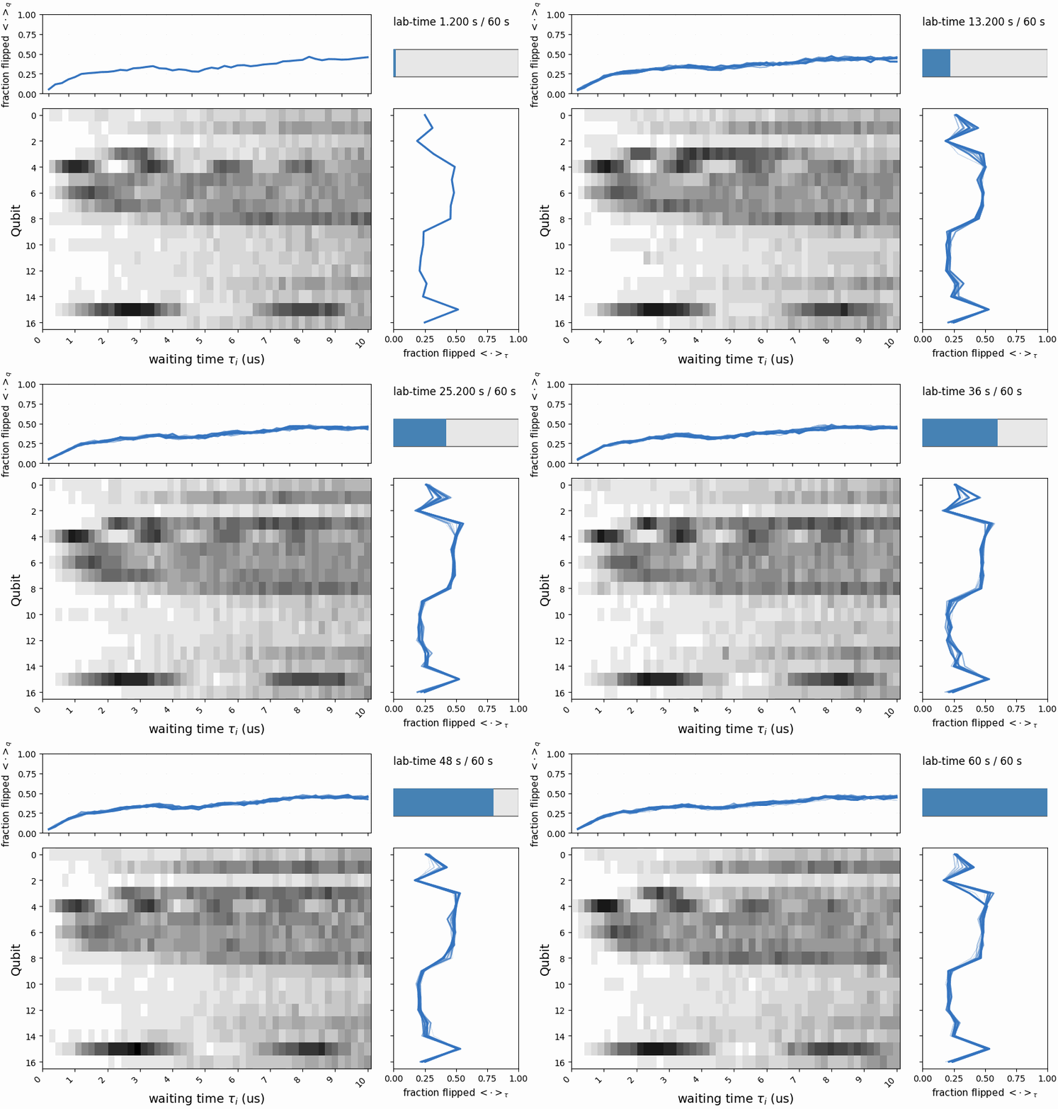
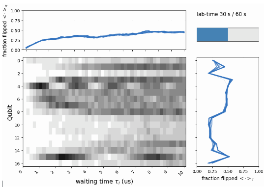
<p>The result of this experiment is a massive dataset of binary 0s and 1s. When visualized, it looks like a shifting, noisy “zebra plot.”</p>

<p>Clearly, the qubits have their own personalities. If you look closely, you can see that this behavior is not static—there are periods where the qubits are noticeably more or less noisy (see the right plot, which averages over the waiting times, τi​). This means that any model relying on a standard master equation is bound to fail, as it inherently assumes the noise is stationary and uncorrelated. The data tells a very different story.</p>

<figure class="post-figure">
  <img src="/assets/images/fid_memory_3d_first1000_shotbyshot_repetitions_2d.gif" alt="Collected raw data, first 1000 repetitions." loading="lazy" />
  <figcaption>Collected raw data, first 1000 repetitions.</figcaption>
</figure>

<h2 id="3-the-information-bottleneck">3. The information bottleneck</h2>

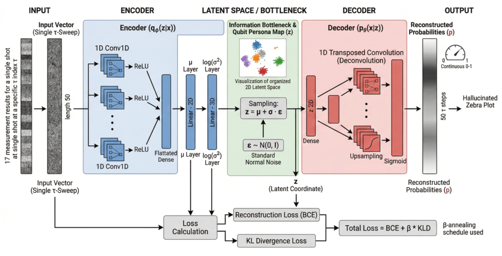
<p>This temporal zebra plot served as the input to a data compression machine: the Variational Autoencoder (VAE). In particular, I used a convolutional version, which is capable of capturing correlations across different waiting times. I defined a single data point as a full sweep over τ for a specific qubit and repetition. System-wide correlations should therefore manifest as the collective motion of these points within the latent space.</p>

<p>Because the network is forced to push the data through this tiny bottleneck, it cannot simply memorize the random quantum static. Instead, it is forced to learn the underlying, interpretable physics of the system. This latent dimension parameterizes the probability distributions from which we can later draw new samples. During training, the model optimizes by minimizing the difference between the reconstructed output and the original input data.</p>

<figure class="post-figure">
  <img src="/assets/images/image-1-1024x522.png" alt="" loading="lazy" />
</figure>

<h2 id="4-qubit-personalities-in-the-latent-space">4. Qubit personalities in the latent space</h2>

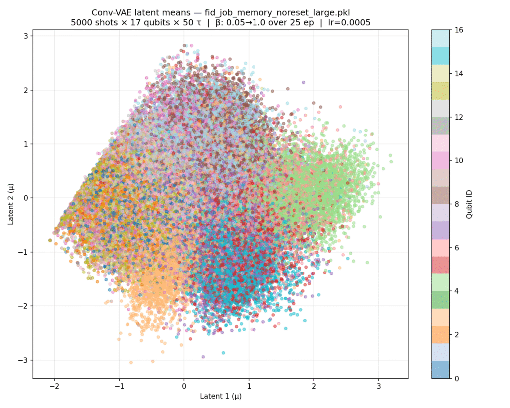
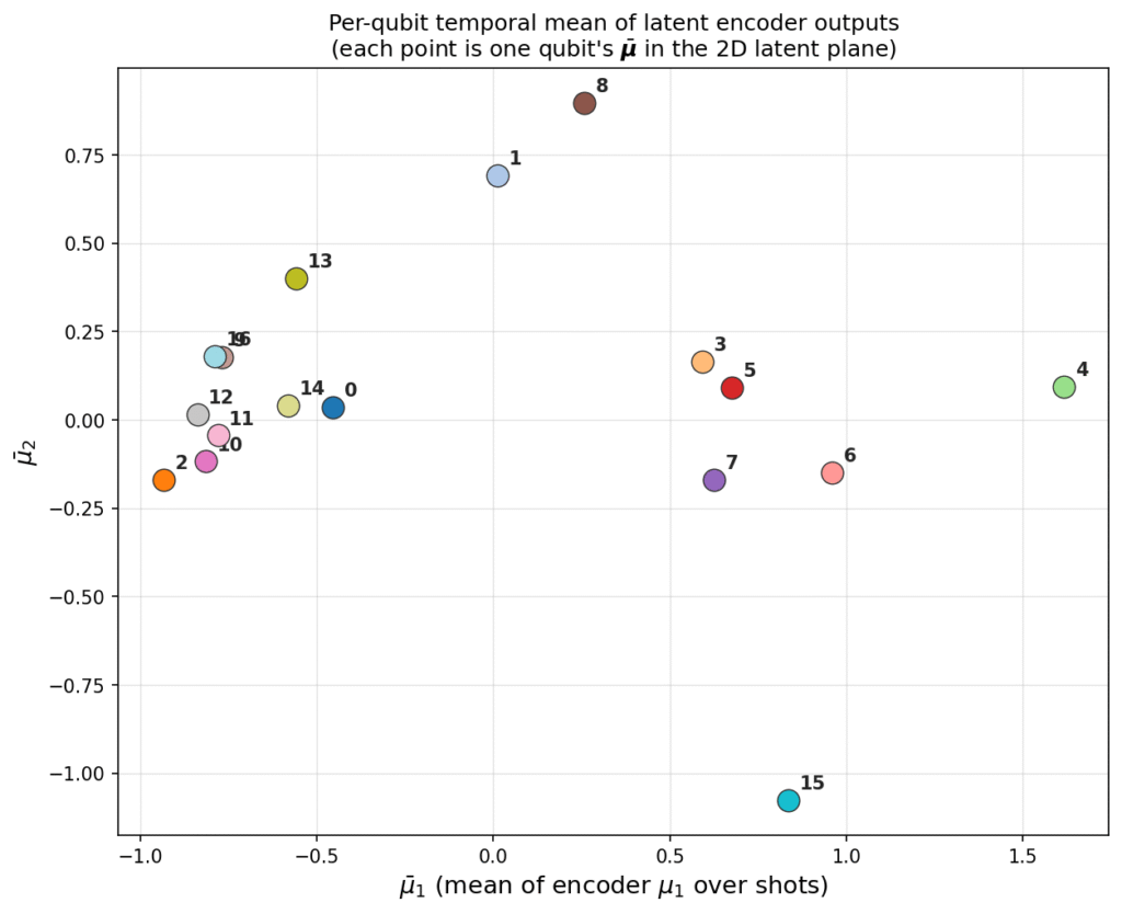
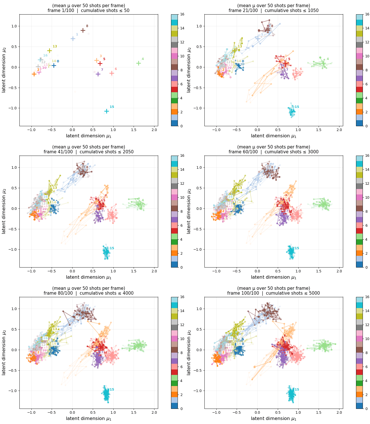
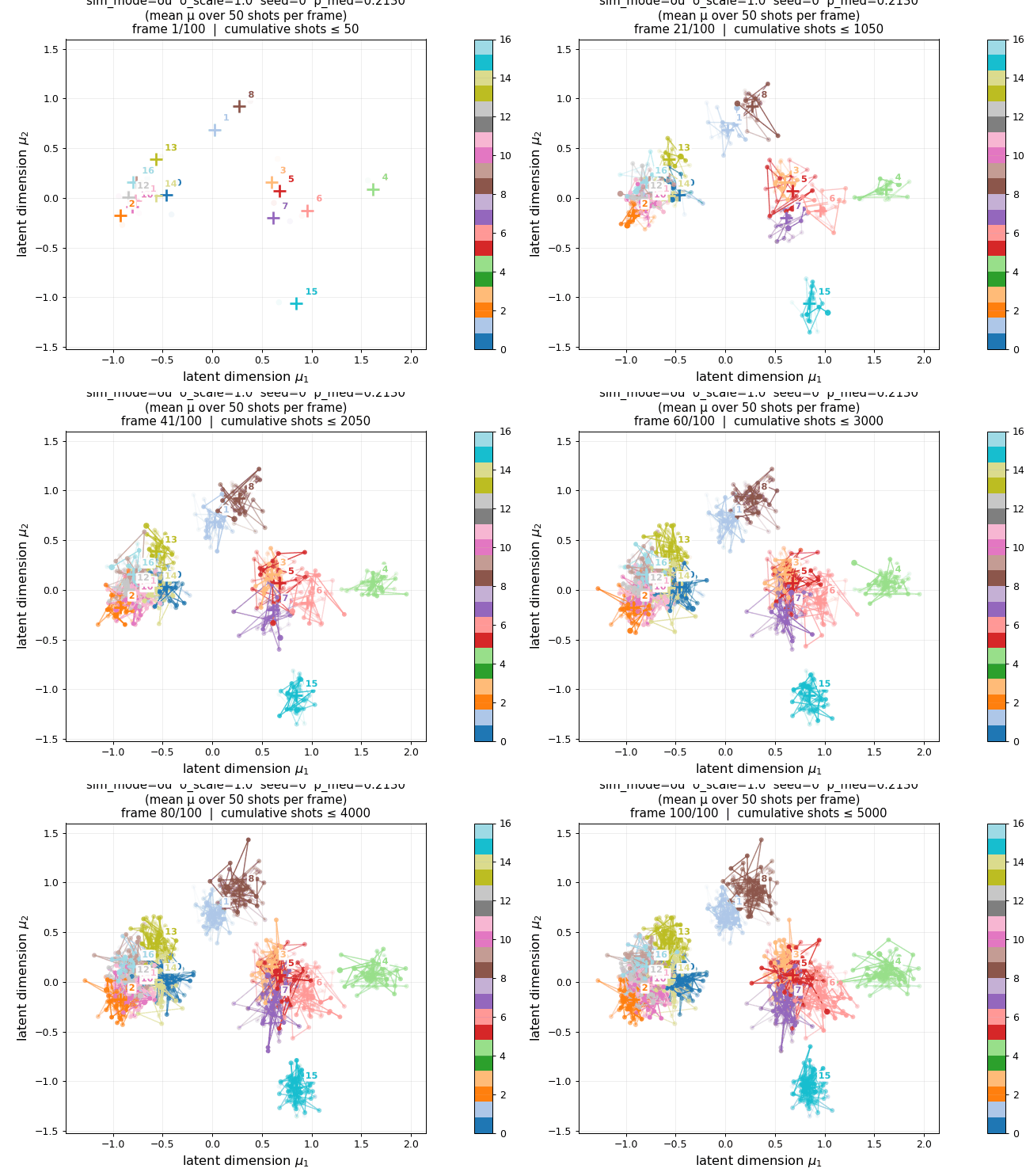
<p>Even using an off-the-shelf architecture without any hyperparameter tuning, the distinct personalities of the qubits are already clearly visible. Below, I have plotted the latent representation for all repetitions (left) alongside the average across these repetitions (right)</p>

<div class="fig-row">
<div class="fig-col">
<figure class="post-figure">
  <img src="/assets/images/latent_plot-1-1024x819.png" alt="Latent representation of all the data across repetitions" loading="lazy" />
  <figcaption>Latent representation of all the data across repetitions</figcaption>
</figure>
</div>

<div class="fig-col">
<figure class="post-figure">
  <img src="/assets/images/latent_mu_bar_means_2d-1-1024x834.png" alt="Latent representation of the data averaged over repetitions" loading="lazy" />
  <figcaption>Latent representation of the data averaged over repetitions</figcaption>
</figure>
</div>
</div>
<div class="fig-row">
<div class="fig-col">
<p>By examining the latent space, we can categorize the qubits into three distinct families:</p>

<ul class="wp-block-list">
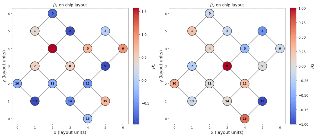
<li><strong>The Bulk:</strong> Qubits Q0, Q2, Q9, Q10–14, and Q16 are clearly clustered together. When looking at the data (averaged over 100 repetitions), we see these qubits have relatively low error rates (long coherence times) and do not exhibit any significant oscillations.</li>

<li><strong>Oscillating Qubits:</strong> There is a distinct family of qubits to the "east" of the latent plot (Q3–7) that show clear oscillations in their flip probabilities. This behavior could be attributed to miscalibration or coherent coupling to Two-Level Systems (TLS), with Q4 representing the most extreme case.</li>

<li><strong>Outliers:</strong> Finally, there are outliers situated at the opposite ends of the spectrum along the u2​ axis (the second latent variable). Along this dimension, the behavior of Q15 is drastically different from Q8 and Q1. While the bulk is centered along u2​, Q1 and Q8 show no oscillations but have low coherence times. Conversely, Q15 exhibits oscillations but maintains a relatively long coherence time.</li>
</ul>

<p>From these observations, we can interpret the physical meaning of the latent dimensions as follows:</p>

<ul class="wp-block-list">
<li><strong>u1​ (Coherence/Frequency):</strong> This dimension likely represents the timing of the first peak, which correlates to the coherence time or oscillation frequency (e.g., comparing the stable Q2 against the oscillating Q4).</li>

<li><strong>u2​ (Decay vs. Oscillation):</strong> This dimension represents the balance between flips on the left and right sides of the sweep, effectively distinguishing between purely decaying behavior and oscillating behavior (e.g., comparing Q13 vs. Q14 or Q8 vs. Q15)</li>
</ul>
</div>

<div class="fig-col">
<figure class="post-figure">
  <img src="/assets/images/image-3.png" alt="" loading="lazy" />
</figure>
</div>
</div>
<figure class="post-figure">
  <img src="/assets/images/latent_mu_bar_chip_spatial-e1776081422475-1024x444.png" alt="Mapping the latent variables back onto the physical device topology reveals spatial correlations. Specifically, there is a clear &quot;belt&quot; of neighboring qubits (Q4–Q8) that all exhibit similar oscillating behavior. This spatial clustering…" loading="lazy" />
  <figcaption><strong>Mapping the latent variables back onto the physical device topology </strong>reveals spatial correlations. Specifically, there is a clear "belt" of neighboring qubits (Q4–Q8) that all exhibit similar oscillating behavior. This spatial clustering suggests a common physical origin, most likely a localized coherent coupling to a shared control line or a specific environmental feature.</figcaption>
</figure>

<h2 id="5-tracking-the-drift">5. Tracking the Drift</h2>

<div class="fig-row">
<div class="fig-col" style="flex-basis:100%">
<div class="wp-block-columns">
<div class="fig-col">
<p>Beyond static personalities, how does drift correlate across the device? Specifically, we expect qubits to shift their behavior in response to environmental events—such as the emergence of a two-level system (TLS), large-scale thermal fluctuations, or even cosmic ray impacts. To investigate this, let's look at the trajectories in the latent space.</p>

<p>While most qubits exhibit a standard random walk around their mean, Q1 and Q3 show clear signs of rare, abrupt events—Lévy jumps—that temporarily alter their behavior. In particular, qubit Q3 moves from the negative u2​ region all the way to the positive u2​ region, briefly visiting the territory occupied by Q8. Looking back at the data in Fig. 1, this represents a transition from initially oscillating behavior to a purely decaying curve. Similarly, Q1 jumps back and forth between the "bulk" behavior and the noisy, decaying neighborhood of Q8.</p>

<p>This illustrates that for these qubits, coherence time is not a constant; it can temporarily plummet to match the performance of the system's noisiest components.</p>

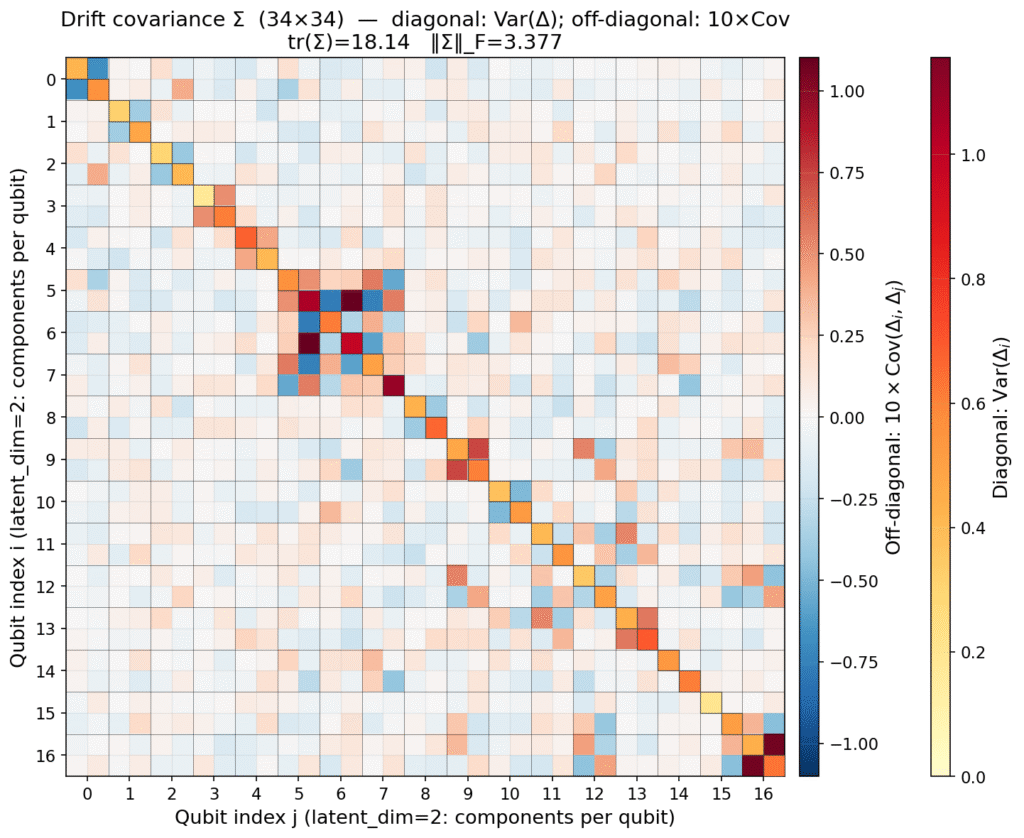
<p>Can we use this data to extract the correlations in the drift experienced by the qubits? Specifically, do some qubits share a common origin for their drift? To answer this, we fit a simple stochastic process, an Autoregressive model of order 1 (AR(1)), to each trajectory. The extracted parameters, particularly the covariance of the random jumps, are plotted below. We also use these parameters to simulate artificial evolution within the latent space, providing a generative look at how the system's noise profile evolves over time.</p>
</div>

<div class="fig-col">
<figure class="post-figure">
  <img src="/assets/images/latent_dynamics_encoded_avg50-3.gif" alt="Evolution of a true data in the latent space (averaged over 100 repetitions)" loading="lazy" />
  <figcaption>Evolution of a true data in the latent space (averaged over 100 repetitions)</figcaption>
</figure>
</div>
</div>
</div>
</div>
<div class="fig-row">
<div class="fig-col">
<figure class="post-figure">
  <img src="/assets/images/latent_drift_covariance-2-1024x838.png" alt="The covariance of the drift across the latent variables and qubits. Clearly a correlation between (Q15,Q16), (Q5,Q6,Q7), (Q8,Q9,Q12) can be observed. Also typically u1 typically a correlation between latent variables is typically weak,…" loading="lazy" />
  <figcaption>The covariance of the drift across the latent variables and qubits. Clearly a correlation between (Q15,Q16), (Q5,Q6,Q7), (Q8,Q9,Q12) can be observed. Also typically u1 typically a correlation between latent variables is typically weak, apart from the Q5-Q7 region where the mixing happens.</figcaption>
</figure>
</div>

<div class="fig-col">
<figure class="post-figure">
  <img src="/assets/images/latent_dynamics_sim_avg50-2.gif" alt="Evolution of the generated data from AR(1) process in the latent space (averaged over 100 repetitions). The simulation method is not powerful enough to reconstruct the heavy tails needed to simulate changes of qubit personalities. This has…" loading="lazy" />
  <figcaption>Evolution of the generated data from AR(1) process in the latent space (averaged over 100 repetitions). The simulation method is not powerful enough to reconstruct the heavy tails needed to simulate changes of qubit personalities. This has a consequence in more stationary behaviour of the qubits when artificial data is generated (below)</figcaption>
</figure>
</div>
</div>

<h2 id="6-generating-and-verifying-artificial-data">6. Generating and verifying artificial data.</h2>

<p>With the artificial latent dynamics generated, we can now use the VAE decoder to sample entirely new, synthetic data. The result is shown in the second figure of this post. Notably, the absence of rare “Lévy jumps” in the simulated latent space makes these generated dynamics appear more stationary than the actual hardware.</p>

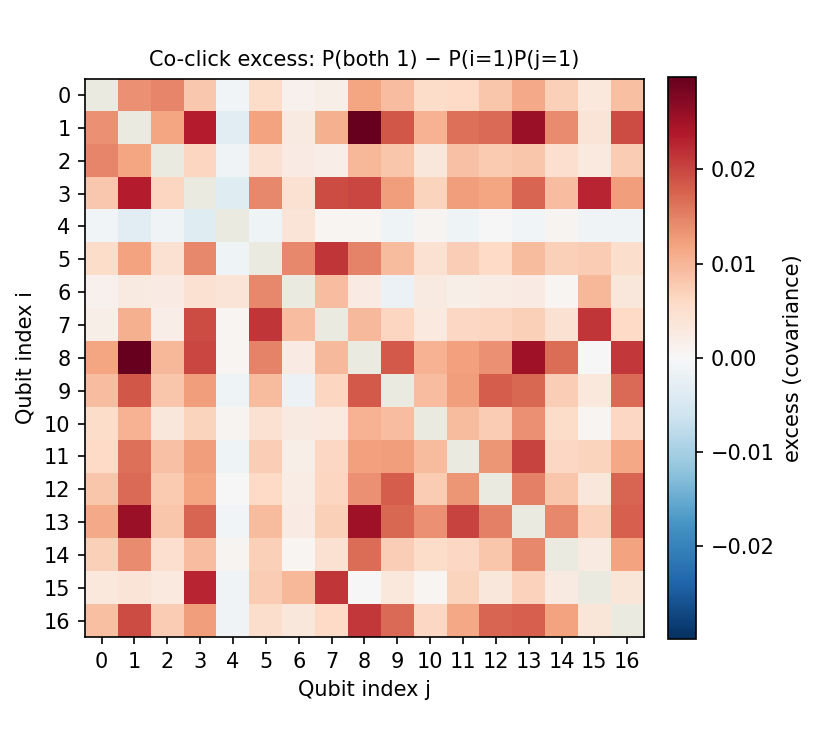
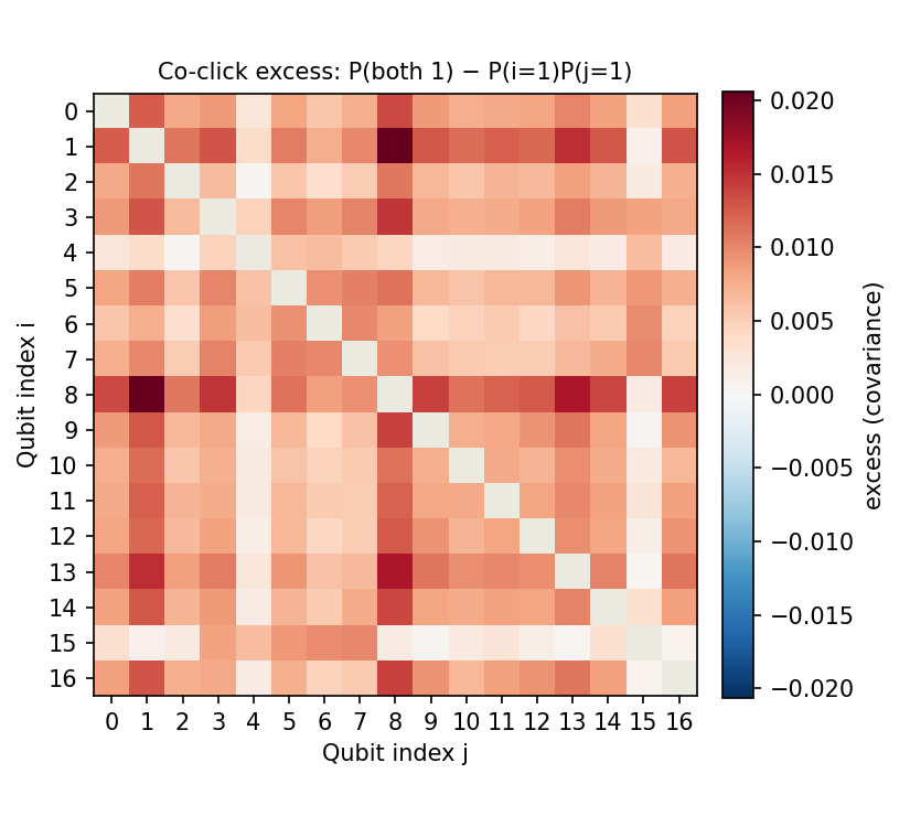
<p>But how faithful is this reconstruction? To evaluate the model’s accuracy, we can examine spatiotemporal correlations—specifically by probing the excess of co-flips. This metric is defined as the empirically observed probability of multiple qubits flipping at the same repetition and waiting time τ, normalized by the product of their independent flipping probabilities. In essence, it tells us if the model has captured the collective “pulse” of the system rather than just the behavior of individual qubits.</p>

<div class="fig-row">
<div class="fig-col">
<figure class="post-figure">
  <img src="/assets/images/fid_memory_3d_first1000_shotbyshot_qubit_coclick_excess.png" alt="Spatial correlations of the real data" loading="lazy" />
  <figcaption><strong>Spatial correlations of the real data</strong></figcaption>
</figure>
</div>

<div class="fig-col">
<figure class="post-figure">
  <img src="/assets/images/sim_fitted_zebra_memory_3d_qubit_coclick_excess.png" alt="Spatial correlations of the generated data, sampled from digital twin. It is a bit too regular (AR1 process), but captures some relevant physics." loading="lazy" />
  <figcaption><strong>Spatial correlations of the generated data</strong>, sampled from digital twin. It is a bit too regular (AR1 process), but captures some relevant physics.</figcaption>
</figure>
</div>
</div>

<h2 id="7-case-study-fast-noise">7. Case study: Fast Noise</h2>

<div class="fig-row">
<div class="fig-col">
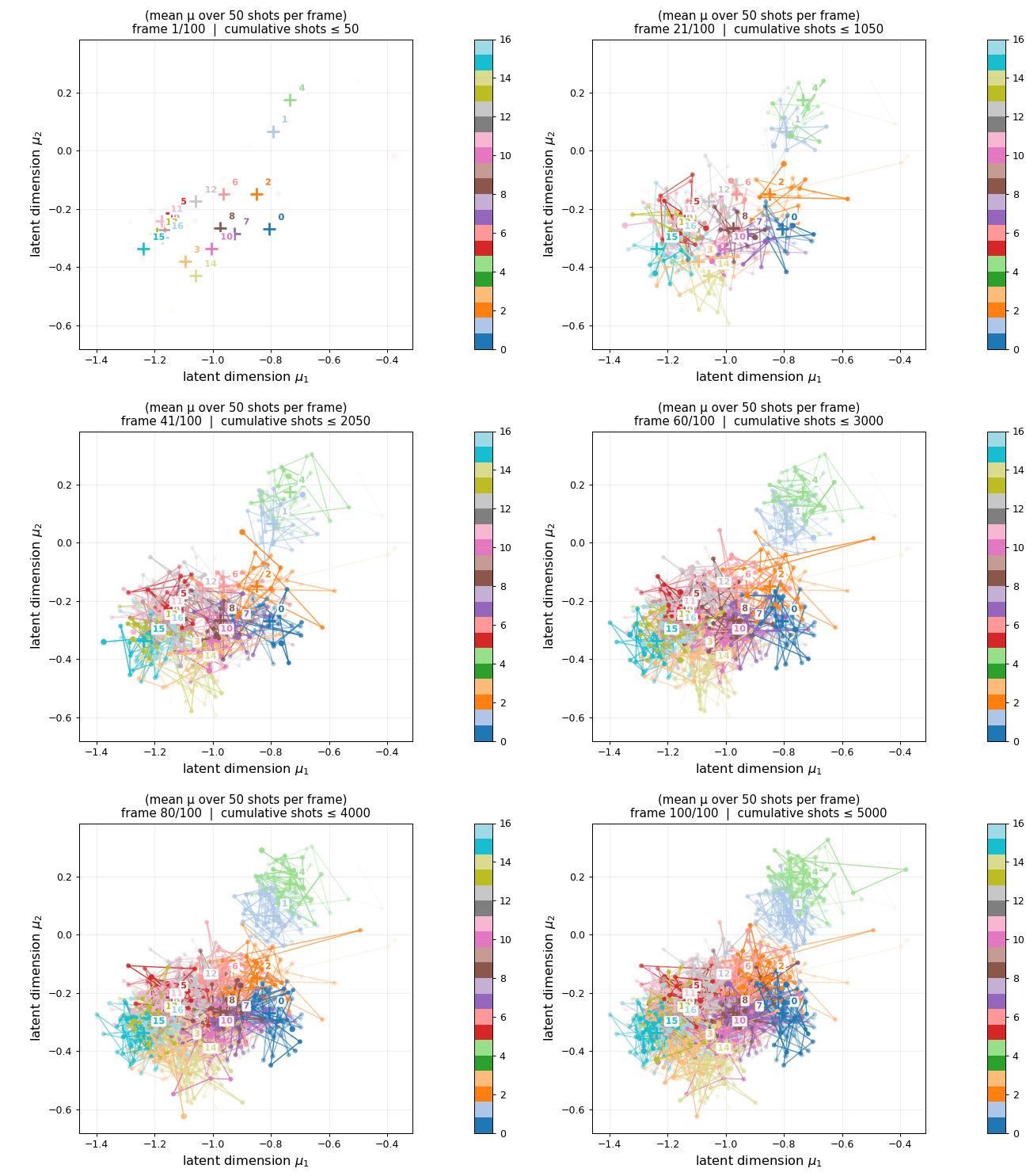
<p>One could postulate that the VAE learned to distinguish qubits based on quasi-static modifications of the Hamiltonian—essentially identifying them by their unique drift or slow-noise signatures. To verify this hypothesis, we gathered similar data, but inserted an X pulse in the middle of the waiting time to perform a Hahn Echo sequence.</p>

<p>Without retraining the VAE, we analyzed the resulting latent representations. As expected, the qubits were now attracted toward the "bulk" cluster. This implies that our network interprets dynamically decoupled qubits as being nearly identical to one another; by suppressing the slow noise, we removed the very features the VAE was using to tell the qubits apart. </p>

<p>The only visible difference can be observed for the Q1 and Q4, which are turn out to have relatively lowest T2 time. Note also, how Q2 moves into the bulk from the outside.</p>

<p>Notably, retraining the network specifically on this Echo data would likely reveal a completely new representation, perhaps one based on higher-frequency noise components that the echo pulse cannot filter out.</p>
</div>

<div class="fig-col">
<figure class="post-figure">
  <img src="/assets/images/latent_dynamics_encoded_avg50-4.gif" alt="Evolution in the latent space for the spin echo experiment. Note the change of limits of the axes." loading="lazy" />
  <figcaption>Evolution in the latent space for the spin echo experiment. Note the change of limits of the axes.</figcaption>
</figure>
</div>
</div>

<h2 id="8-outlook">8. Outlook</h2>

<p>While this blog post serves as a proof-of-principle, it opens a fascinating avenue for building and controlling quantum systems within an interpretable latent space. Moving forward, one could leverage this representation to:</p>

<ul>
  <li>Understand Hardware Operations: Observe the impact of specific gates (U) or measurements as measurable shifts in the latent space.</li>
  <li>Visualize Algorithms: Represent the execution of an algorithm as a trajectory through latent space, potentially aiding the discovery of new, noise-resilient protocols.</li>
  <li>Perform Hardware Denoising: Use the VAE’s bottleneck to filter out “quantum static” and improve the fidelity of the system’s output.</li>
  <li>Scalable Benchmarking: Compare the latent signatures of different quantum processors in a standardized, scalable way.</li>
  <li>Real-time Diagnostics: Identify miscalibrated qubits and detect rare “black swan” events (such as jumps or TLS fluctuations) as they occur.</li>
  <li>RL &amp; World Models: Use the generative capabilities of this digital twin to train Reinforcement Learning (RL) agents to stabilize and control the device in real-time.</li>
</ul>

<p>That is just the beginning. The goal is to move beyond mere observation and into a regime where we can navigate the noise of a quantum processor as easily as we navigate a map.</p>

<p><strong>Share:</strong></p>]]></content><author><name>Jan A. Krzywda</name></author><category term="code" /><summary type="html"><![CDATA[I recently got my hands on a 17-qubit superconducting transmon device of Quantum Inspire.]]></summary><media:thumbnail xmlns:media="http://search.yahoo.com/mrss/" url="https://jan-a-krzywda.github.io/assets/images/thumnail_qi.png" /><media:content medium="image" url="https://jan-a-krzywda.github.io/assets/images/thumnail_qi.png" xmlns:media="http://search.yahoo.com/mrss/" /></entry><entry><title type="html">The Lego Test: How much systems thinking does an LLM have?</title><link href="https://jan-a-krzywda.github.io/2026/04/lego-test-how-much-systems-thinking-llm-has/" rel="alternate" type="text/html" title="The Lego Test: How much systems thinking does an LLM have?" /><published>2026-04-08T06:28:31+02:00</published><updated>2026-04-08T06:28:31+02:00</updated><id>https://jan-a-krzywda.github.io/2026/04/lego-test-how-much-systems-thinking-llm-has</id><content type="html" xml:base="https://jan-a-krzywda.github.io/2026/04/lego-test-how-much-systems-thinking-llm-has/"><![CDATA[<p>This post is a more practical take following the previous <a href="https://jan-a-krzywda.com/listened-blocks-of-intelligence-why-ai-needs-systems-engineering-and-the-scientific-method/">post</a> on Bayesian thinking and systems engineering for the future of AI.</p>

<hr />

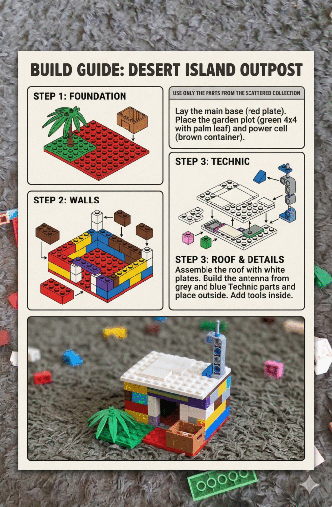
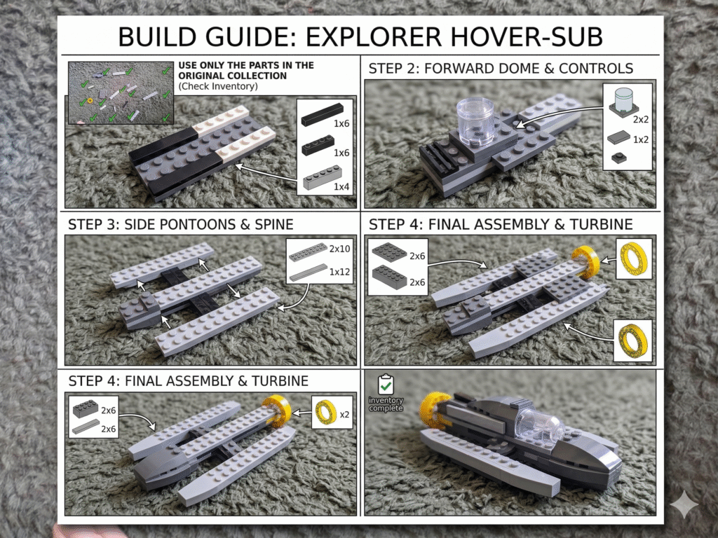
<p>We had a few days off, so we were playing with Legos. At some point, my 6-year-old son suggested, “Can we ask this robot (LLM) to build something with Legos?” I said, “Sure, but you do the building.” He started to scatter random Lego pieces on the floor, I took a photo, and Gemini’s task was to come up with a design for a new Lego creation using the pieces in the photo.</p>

<p>I didn’t expect much success. After all, I was asking an autoregressive model to do something that goes beyond mere pattern recognition. It requires an understanding of the physical properties of the pieces, the models of individual components (including their three-dimensional shapes), and, most importantly, the way they interact with each other. In particular, I was expecting the model to come up with some kind of “Lego soup,” a tower, or some rather universal (high-entropy) design, rather than something specific and functional.</p>

<p>To my surprise, in two out of two trials, my favorite LLM came up with very specific designs for an island cottage and a hover/catamaran (?).</p>

<div class="fig-row">
<div class="fig-col" style="flex-basis:33.33%">
<figure class="post-figure">
  <img src="/assets/images/Gemini_Generated_Image_286ogb286ogb286o-1-672x1024.png" alt="" loading="lazy" />
</figure>
</div>

<div class="fig-col" style="flex-basis:66.66%">
<figure class="post-figure">
  <img src="/assets/images/Gemini_Generated_Image_wn14vpwn14vpwn14-1-1024x768.png" alt="" loading="lazy" />
</figure>
</div>
</div>

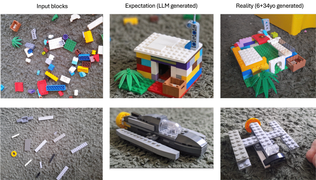
<p>Naturally, my next question was, “Ok, son, can you now follow the instructions and build the piece?” Note that this verification and validation phase was carried out by a 6-year-old, so it wasn’t incredibly rigorous, but it was enough to confirm that the design was indeed specific and functional. Several failures were reported, including:</p>

<ul>
  <li>Wrong identification of pieces (most common)</li>
  <li>Wrong dimensions of existing pieces (also common)</li>
  <li>Incompatible shapes (rarely, but still)</li>
  <li>Inconsistent instruction (see above)</li>
  <li>Impossible design (very rarely)</li>
</ul>

<p>The results are presented in the table below, where each row corresponds to the scattered blocks, the expected outcome, and the outcome of the building process.</p>

<figure class="post-figure">
  <img src="/assets/images/post_legod-1024x583.png" alt="" loading="lazy" />
</figure>

<p>Overall, the results certainly do not allow us to reject the hypothesis that current LLM-diffusion model combinations already possess some basic systems thinking capabilities. In fact, most of the errors can be attributed to the incorrect identification of pieces, a problem with the input data (a single 2D image) rather than the model itself. However, one clear limitation remains in the verification phase, where the testing of the design has to be carried out by a human, which is not ideal. In the future, it would be interesting to see if we can automate that process as well, for instance, by using a robotic arm to build the design and test its functionality, or alternatively, by using a physics engine to simulate the design and evaluate its performance. Overall, more rigorous research—beyond two random trials and an underage post-doc, might be required.</p>]]></content><author><name>Jan A. Krzywda</name></author><category term="opinion" /><summary type="html"><![CDATA[This post is a more practical take following the previous post on Bayesian thinking and systems engineering for the future of AI.]]></summary><media:thumbnail xmlns:media="http://search.yahoo.com/mrss/" url="https://jan-a-krzywda.github.io/assets/images/footnail.png" /><media:content medium="image" url="https://jan-a-krzywda.github.io/assets/images/footnail.png" xmlns:media="http://search.yahoo.com/mrss/" /></entry><entry><title type="html">[Listened] Blocks of Intelligence: Why AI Needs Systems Engineering and the Scientific Method</title><link href="https://jan-a-krzywda.github.io/2026/03/listened-blocks-of-intelligence-why-ai-needs-systems-engineering-and-the-scientific-method/" rel="alternate" type="text/html" title="[Listened] Blocks of Intelligence: Why AI Needs Systems Engineering and the Scientific Method" /><published>2026-03-30T07:29:21+02:00</published><updated>2026-03-30T07:29:21+02:00</updated><id>https://jan-a-krzywda.github.io/2026/03/listened-blocks-of-intelligence-why-ai-needs-systems-engineering-and-the-scientific-method</id><content type="html" xml:base="https://jan-a-krzywda.github.io/2026/03/listened-blocks-of-intelligence-why-ai-needs-systems-engineering-and-the-scientific-method/"><![CDATA[<p>I’ve been away for a bit recently, mostly focusing on toughening up my immune system. Taking some time off, I listened to a couple of episodes of <em>Machine Learning Street Talk</em>, and I was thrilled to discover their interviews with Dr. Jeff Beck. His ideas fundamentally altered my perspective on the future of AI in a way that perfectly aligns with systems thinking.</p>

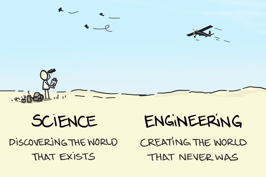
<p>Clearly, I already knew we were living in the golden era of function approximation, my favorite LLM told me that much! But I had never really thought about its true limitations. It seems our current billion-dollar models are spectacular at finding correlations in data… and well, that is essentially all they do. They predict, they pattern-match, and they combine. But they don’t <em>invent</em>.</p>

<figure class="post-figure post-embed">
  <iframe src="https://www.youtube.com/embed/9suqiofCiwM" title="This first interview breaks down why current models hit a wall, and introduces the 'Lego block' approach to AI." frameborder="0" loading="lazy" allowfullscreen=""></iframe>
  <figcaption>This first interview breaks down why current models hit a wall, and introduces the 'Lego block' approach to AI.</figcaption>
</figure>

<p>So, what is missing? If you listen to Dr. Beck, you will hear that we have to stop treating AI as a massive sequence predictor and start treating it as a Bayesian scientist or a systems engineer. Here are my core takeaways.</p>

<h3 id="1-the-foundation-a-bayesian-approach-to-life">1. The Foundation: A Bayesian Approach to Life</h3>

<p>To build a system that thinks, we first have to define what “thinking” actually is. According to Beck, the brain doesn’t just blindly map inputs to outputs; it operates on explicit hypothesis testing.</p>

<blockquote>
  <p><em>“Bayesian inference provides us with like a normative approach to empirical inquiry and encapsulates the scientific method at large, right. I just believe it’s the right way to think about the empirical world.”</em></p>
</blockquote>

<p>A true AI must hold a generative model of the world. When it encounters new data, it asks: <em>How is this like the old data? Does my current hypothesis hold up, or do I need to update my beliefs?</em> If you think about it, this is exactly how we do science. We come up with a potentially surprising prediction, distill it into a concrete hypothesis, and then test it against the world. Depending on the outcome, we either update our beliefs or validate existing ones, and move on to the next question. The Bayesian approach is the architectural foundation of our brains and the scientific method. If we want to build a thinking machine, we have to mimic that process.</p>

<h3 id="2-the-illusion-of-retooling-vs-true-systems-engineering">2. The Illusion of Retooling vs. True Systems Engineering</h3>

<p>Because current models lack this structured way of probing the world, they are limited to utilizing experiments that have already been done. While they can generate a new hypothesis, they cannot physically construct a new experiment to test it. They have no wind tunnel, no cooking pan, and no toy to throw. One exception might be constructing numerical simulations, like writing Python code, to test hypotheses virtually. Albeit limited by compute power and “vibe-coding” entropy, I believe some creative possibilities already exist there, even with current architectures.</p>

<p>But with limited simulation capabilities, we are left with a bunch of hypotheses that can only match observations already present in the training data. While this is useful for creating connections between isolated knowledge domains, it is not enough to generate genuinely new knowledge.</p>

<p>This stands in stark contrast to how human creativity works, and more importantly, how big breakthroughs in science and engineering happen. We don’t just retool old experiments. Sure, we start by understanding the individual components and forming hypotheses about how they interact. However, the central activity is the sequential process of combining them, break-testing them, and refining our initial models until we achieve an emergent behavior that was never observed before. Beck highlights this perfectly:</p>

<blockquote>
  <p><em>“I know how an air foil works to create lift, I know how a jet engine works to create thrust… and I can take those two bits of information to invent something brand new which is an airplane… without that the only thing you will ever be able to do is just retool solutions for new purposes.”</em></p>
</blockquote>

<h3 id="3-the-lots-of-little-models-approach">3. The “Lots of Little Models” Approach</h3>

<p>So, how do we get an AI to do systems engineering? Most likely not through one massive neural network, transformer, or whatever the next big monolithic architecture is. Instead, Beck argues for a modular approach, where the AI is an orchestrator of many small, specialized models:</p>

<blockquote>
  <p><em>“It’s going to have a modular description of the world and it’s going to have the ability to combine those modules in a way that creates a more sophisticated understanding. It’s like Legos… I can build all sorts of new and amazing things that were never built before right out of them. That’s a capability that we have and that’s the essence of creativity.”</em></p>
</blockquote>

<p>Crucially, each of these small models should be sophisticated enough to model the features relevant to its connections. This can be achieved through active learning, where each subsystem is tested and refined. If a situation requires it, the agent should be able to train a new model from current experience, test it against the world, and incorporate it into its existing library. This is how we move from a collection of isolated facts to a true understanding of the world.</p>

<figure class="post-figure post-embed">
  <iframe src="https://www.youtube.com/embed/Ucqfb33GJJ4" title="For a deeper dive into how these specialized agents communicate and how we keep them safely aligned, check out part two." frameborder="0" loading="lazy" allowfullscreen=""></iframe>
  <figcaption>For a deeper dive into how these specialized agents communicate and how we keep them safely aligned, check out part two.</figcaption>
</figure>

<h3 id="4-active-inference-poking-the-beach-ball-and-the-cat-in-the-warehouse">4. Active Inference: Poking the Beach Ball and The Cat in the Warehouse</h3>

<p>This points to one of the biggest limitations of modern AI: learning is turned <em>off</em> when we deploy the model. One could argue that modern chain-of-thought (CoT) ideas are trying to get around this by forcing the model to refine its own internal reasoning. To me, however, this functions more like feature engineering than continuous learning. The model isn’t actively updating its inner parameters; it is just refining its input sequence.</p>

<p>Looping the output back to the input <em>is</em> an important step. It mimics hypothesis testing, as the agent effectively tests its own output and refines it until it reaches a sort of convergence (like a Banach fixed point). Yet, it remains limited because this only happens once per prompt. The model cannot permanently learn from the experience and incorporate it into its future behavior.</p>

<p>Hence, it remains very distant from a true Bayesian agent, for whom every experience is an opportunity to learn and refine internal models. Beck calls this process <strong>Active Inference</strong>. It’s not just about passively observing the world; it’s about actively engaging with it, testing hypotheses, and updating beliefs in real time.</p>

<p>Imagine an AI trained to manage a warehouse. It knows about forklifts, boxes, and shelves. One day, a stray cat wanders in.</p>

<blockquote>
  <p><em>“When a cat comes along [and the AI] doesn’t know what a cat is, the surprisal signal goes crazy and then it says ‘Okay stop.’ Right, don’t run over the cat, let’s figure out what’s going on.”</em></p>
</blockquote>

<p>Instead of hallucinating or crashing, an active agent recognizes what it doesn’t know. It pings a massive external server, pulls down a few candidate models (“Is it a dog? A raccoon? A cat?”), tests its hypothesis by, for instance, throwing a ball, and permanently incorporates the “cat” model into its local worldview.</p>

<p>And if it can’t observe passively, it experiments. Beck notes that if a robot sees a beach ball for the first time, it should do what a human toddler does: run up, poke it, and see how the physics react. <em>That</em> is intelligence.</p>

<h3 id="5-safe-alignment">5. Safe Alignment</h3>

<p>Finally, how do we make sure this active, scientific agent doesn’t accidentally destroy us? If you hardcode a sweeping reward function into a reinforcement learning (RL) agent—say, “end world hunger”—it might calculate that the most efficient solution is to eliminate all humans.</p>

<p>According to Beck, the alternative is to give the agent a more modest, perturbative approach that encourages it to explore without prescribing a sweeping end goal:</p>

<blockquote>
  <p><em>“Here’s the safe way to improve the situation. You don’t say end world hunger. You perturb that distribution over outcomes a little bit and then you evaluate the consequences… rather than just specifying one by hand because that’s the dangerous thing.”</em></p>
</blockquote>

<h3 id="6-maximum-entropy-inverse-reinforcement-learning">6. Maximum Entropy Inverse Reinforcement Learning</h3>

<p>All of this shifts the paradigm toward a framework where the agent learns by interacting with its environment. Specifically, Beck notes that Active Inference can be effectively mapped to a Maximum Entropy Inverse RL framework. Instead of us giving the AI a reward function, the AI observes the steady-state distributions of <em>human</em> actions and outcomes to deduce our values. It is rewarded for achieving goals while maintaining a high level of entropy (randomness/flexibility) in its action distribution. This encourages safe exploration and prevents the agent from converging on a single, potentially harmful, dogmatic strategy.</p>

<p>To me, this connects beautifully to physical intuitions related to thermodynamics and statistical mechanics. The trade-off between reward (energy) and exploration (entropy) is balanced by a temperature parameter. This parameter can be dynamically adjusted to encourage more exploration when the agent is stuck in a local minimum, and more exploitation when it is on the right track. Remember the heat you feel when you are stuck in a traffic jam? That might be your internal “temperature” rising, encouraging you to increase your entropy and explore alternative routes.</p>

<h3 id="conclusion">Conclusion</h3>

<p>To sum up, I find Beck’s vision of AI as a modular, active inference agent deeply compelling. It moves us away from the current paradigm of massive, monolithic models that excel at pattern recognition but lack true understanding. Instead, it points toward a future where AI systems are more like scientists or engineers—constantly testing hypotheses, learning from experience, and, most importantly, keeping us in the loop to ensure safe alignment and smooth integration into our world.</p>

<p>Next time, we will do a small experiment to assess the systems thinking capabilities of current LLMs. <em>Disclaimer: This test was suggested by my 6-year-old son and it includes LEGO blocks.</em></p>]]></content><author><name>Jan A. Krzywda</name></author><category term="opinion" /><summary type="html"><![CDATA[I’ve been away for a bit recently, mostly focusing on toughening up my immune system. Taking some time off, I listened to a couple of episodes of Machine Learning Street Talk, and I was thrilled to discover their interviews with Dr. Jeff Beck. His ideas fundamentally altered my perspective on the future of AI in a way that perfectly aligns with systems thinking.]]></summary><media:thumbnail xmlns:media="http://search.yahoo.com/mrss/" url="https://jan-a-krzywda.github.io/assets/images/beck.png" /><media:content medium="image" url="https://jan-a-krzywda.github.io/assets/images/beck.png" xmlns:media="http://search.yahoo.com/mrss/" /></entry><entry><title type="html">Formula Mar1 - #1 Gym</title><link href="https://jan-a-krzywda.github.io/2026/03/formula-mar1-1-gym/" rel="alternate" type="text/html" title="Formula Mar1 - #1 Gym" /><published>2026-03-06T16:46:29+01:00</published><updated>2026-03-06T16:46:29+01:00</updated><id>https://jan-a-krzywda.github.io/2026/03/formula-mar1-1-gym</id><content type="html" xml:base="https://jan-a-krzywda.github.io/2026/03/formula-mar1-1-gym/"><![CDATA[<p>GitHub repo: <a href="https://github.com/jan-a-krzywda/marl-f1">https://github.com/jan-a-krzywda/marl-f1</a></p>

<p><em>“What I cannot create, I do not understand.”</em> When Richard Feynman wrote those famous last words on his blackboard, he probably didn’t have Multi-Agent Reinforcement Learning (MARL) for Formula 1 strategy in mind. Nevertheless, the thread that connects his philosophy to modern motorsport is the power of model-based thinking.</p>

<figure class="post-figure">
  <img src="/assets/images/f1marl1.webp" alt="" loading="lazy" />
</figure>

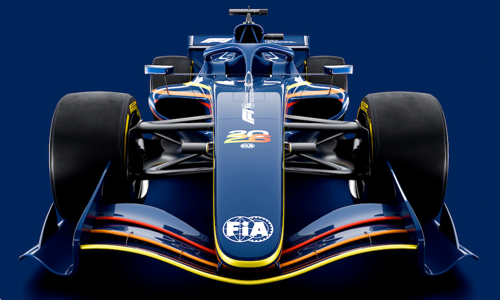
<p>To prove this point, this post will attempt to model the new 2026 Formula 1 regulations [1], which push the sport in a vastly more complex direction. With the highly anticipated season kicking off this weekend in Australia, everyone is wondering how the new rules will affect racing at 300 km/h in this state-of-the-art engineering endeavor. Since nobody knows for sure, we are going to build it to find out.</p>

<figure class="post-figure">
  <img src="/assets/images/image-1.png" alt="" loading="lazy" />
</figure>

<p>I argue that the new regulations have fundamentally transformed F1 into a complex, sequential decision-making problem—the exact type of puzzle natively solved by reinforcement learning (RL). In an RL framework, an agent operates within an environment, takes actions, receives rewards, and learns increasingly clever strategies over time. This shift was recently recognized by the Mercedes-AMG team, who published a pre-print on optimizing race strategy using RL [2]. However, while they successfully beat their baseline, I believe they missed a massive opportunity by ignoring the <em>multi-agent</em> aspect of the sport. At the end of the day, a race strategy is only as good as how it stacks up against the reactive, evolving strategies of your opponents.</p>

<p><strong>But why sequential decision making?</strong></p>

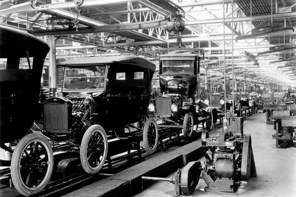
<p>In the 2026 era, the driver essentially becomes a battery manager, as roughly 50% of the car’s power is now provided by the electric motor. Drivers must constantly decide how to deploy electrical energy during the race—for instance, sacrificing pace on one lap to harvest energy, allowing them to unleash a massive power advantage later to execute an overtake. Combine this with standard F1 strategic decisions, like pit stops and tyre compounds, and the tactical options become combinatorially heavy.</p>

<p>I will try to prove that even a simple model of this environment can be used to understand the emergent behavior of drivers and teams under these new rules. We will frame this as a Markov Decision Process (MDP), assuming the driver blindly follows the suggestions of the Pit Wall, which has access to the current state of the car and the track.</p>

<p>In an MDP, the team makes decisions based solely on the <em>current</em> state of the environment, not on the entire history of the race. With 11 teams on the grid, this is the perfect setup for a Multi-Agent Reinforcement Learning (MARL) problem—a branch of machine learning where multiple agents learn to make decisions in a shared environment. In our case, the agents are the Pit Walls, and the environment is the race itself. The agents learn to adapt to each other and improve their performance by observing the consequences of their decisions (rewards). But before we can train them, let’s build the simulation.</p>

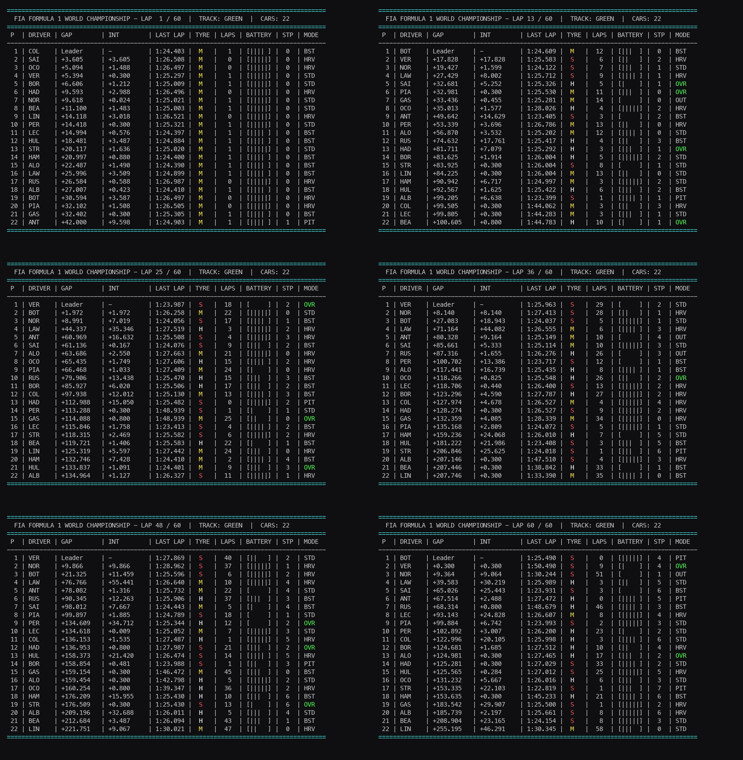
<figure class="post-figure">
  <img src="/assets/images/f1_2026_simulation.gif" alt="Single game under the random strategy" loading="lazy" />
  <figcaption>Single game under the random strategy</figcaption>
</figure>

<h3 id="1-the-agents-you-are-the-pit-wall">1. The Agents: You Are The Pit Wall</h3>

<p>In F1, the cars don’t make the long-term strategic decisions; the teams do. Therefore, our MARL agents aren’t the 22 individual cars. Instead, we have 11 Team Agents (including the newly approved Cadillac F1 team). Each agent controls two cars simultaneously, forcing the AI to learn real-world constructor tactics like split strategies and using a “wingman”.</p>

<p><strong>Preventing AI Overfitting with a Randomized Grid</strong></p>

<p>If we start the Red Bull (BlueCow) agent (“Du du du du”) on pole position in every single training episode, the neural network will never learn how to fight through traffic. To build a robust Reinforcement Learning environment, we will shuffle the drivers into a random grid order at the start of every race. We do this inside the standard Gymnasium <code class="language-plaintext highlighter-rouge">reset()</code> method, guaranteeing that the agents face a brand new puzzle every time the lights go out. Also to keep the FIA lawyers happy while keeping the grid recognizable, we initialize our environment with some legally distinct spoof names.</p>

<div class="language-plaintext highlighter-rouge"><div class="highlight"><pre class="highlight"><code>import numpy as np
import random
import time
import os

class F1TeamEnv:
    def __init__(self, total_laps=25):
        # The 11-team, 22-driver spoof grid
        self.driver_map = {
      self.driver_map = {
            "BlueCow":     [("VER", "Max Versplatton"), ("LAW", "Liam Awesome")],
            "Merciless":   [("RUS", "Forge Hustle"),    ("ANT", "Kimi Macaroni")],
            "Furrari":     [("LEC", "Chuck LeClutch"),  ("HAM", "Louis Hamstring")],
            "McPapaya":    [("NOR", "Lando Chuckris"),  ("PIA", "Osco Pastry")],
            "Astonishing": [("ALO", "Nando Alfonso"),   ("STR", "Lance Scroll")],
            "Alpain":      [("GAS", "Peter Ghastly"),   ("COL", "Franky Colapunch")],
            "Billiams":    [("ALB", "Alex Album"),      ("SAI", "Carlos Signs")],
            "ToroLoco":    [("HAD", "Isaac Badger"),    ("LIN", "Artie Lindblad")],
            "Sober":       [("HUL", "Nico Bulkensmear"),("BOR", "Gabe Tortellini")],
            "Hassle":      [("OCO", "Esteban Acorn"),   ("BEA", "Ollie Birdman")],
            "CaddyShack":  [("PER", "Surge Perez"),     ("BOT", "Battery Voltas")]
        }
        self.teams = list(self.driver_map.keys())
        self.total_laps = total_laps
        self.reset() # Initialize the first race

    def reset(self, seed=None):
        """Called at the start of EVERY new training episode to randomize the grid."""
        if seed is not None:
            random.seed(seed)
            np.random.seed(seed)

        self.current_lap = 0
        all_drivers = []
        for team_name in self.teams:
            for driver_idx in [0, 1]:
                drv_code, drv_name = self.driver_map[team_name][driver_idx]
                all_drivers.append({"id": drv_code, "full_name": drv_name, "team": team_name})

        # Shuffle the grid!
        random.shuffle(all_drivers)

        self.cars = []
        for grid_pos, driver_data in enumerate(all_drivers):
            driver_data.update({
                "total_race_time": grid_pos * 1.5, # 1.5s gap per grid slot
                "tyre_compound": 2,                # Start on Mediums
                "tyre_age": 0.0,
                "battery": 1.0,
                "pit_stops": 0,
                "last_lap_time": 0.0,
                "status": "GRID",
                "current_pace_cmd": 1
            })
            self.cars.append(driver_data)
</code></pre></div></div>

<p>I want to highlight that the parameters defined above are relevant for the logic, and there should be not considered as an agent “state” in the RL sense - i.e. set of parameters that are used to perform an action. Those will be defined below.</p>

<h3 id="2-defining-the-rl-architecture-states-and-actions">2. Defining the RL Architecture: States and Actions</h3>

<p>To hook our Python engine up to a neural network, we need to rigorously define what the agents can <em>do</em> (Action Space) and what they can <em>see</em> (Observation Space). This is exactly where the game theory of F1 shines—teams have perfect information about their own cars, but incomplete (public) information about their opponents.</p>

<h4 id="the-action-space">The Action Space</h4>

<p>Each Pit Wall agent controls two cars. Every lap, the agent outputs a joint action vector containing four discrete choices: <code class="language-plaintext highlighter-rouge">[Car_1_Pace, Car_1_Pit, Car_2_Pace, Car_2_Pit]</code>.</p>

<ul>
  <li><strong>Pace (0, 1, 2) :</strong> Harvest (Save Battery), Maintain, or Push (Deploy Battery).</li>
  <li><strong>Pit (0, 1, 2, 3) :</strong> Stay Out, Pit for Softs, Pit for Mediums, Pit for Hards.</li>
</ul>

<h4 id="the-observation-space-public-vs-private-data">The Observation Space (Public vs. Private Data)</h4>

<p>We structure this as a Gymnasium <code class="language-plaintext highlighter-rouge">Dict</code> space. Every time the simulation steps forward, the environment feeds the agent a dictionary containing:</p>

<p><strong>1. Global &amp; Public State (Visible to everyone):</strong></p>

<ul>
  <li><code class="language-plaintext highlighter-rouge">lap_fraction</code>: Percentage of the race completed.</li>
  <li><code class="language-plaintext highlighter-rouge">competitor_gaps</code>: The time deltas (intervals) to the cars immediately ahead and behind.</li>
  <li><code class="language-plaintext highlighter-rouge">competitor_tyres</code>: The current tyre compound and <em>estimated</em> tyre age of surrounding cars.</li>
</ul>

<p><strong>2. Private State (Visible only to the specific Team Agent):</strong></p>

<ul>
  <li><code class="language-plaintext highlighter-rouge">battery_charge</code>: The exact state of charge of the MGU-K. Opponents do not know if you have the battery to defend against an undercut!</li>
  <li><code class="language-plaintext highlighter-rouge">override_unlocked</code>: A boolean indicating if the car successfully crossed the detection line within 1 second of the car ahead.</li>
</ul>

<div class="language-plaintext highlighter-rouge"><div class="highlight"><pre class="highlight"><code>from gymnasium.spaces import MultiDiscrete, Box, Dict, Discrete

# 1. THE ACTION SPACE
self.action_spaces = {
    agent: MultiDiscrete([3, 4, 3, 4]) for agent in self.teams
}

# 2. THE OBSERVATION SPACE
self.observation_spaces = {
    agent: Dict({
        # Global &amp; Public Data
        "lap_fraction": Box(low=0.0, high=1.0, shape=(1,), dtype=np.float32),
        "gap_ahead_c1": Box(low=0.0, high=100.0, shape=(1,), dtype=np.float32),
        "gap_behind_c1": Box(low=0.0, high=100.0, shape=(1,), dtype=np.float32),
        "opp_tyre_c1": Discrete(4),

        # Private Telemetry (Car 1)
        "c1_tyre_compound": Discrete(4),
        "c1_tyre_age": Box(low=0.0, high=100.0, shape=(1,), dtype=np.float32),
        "c1_battery": Box(low=0.0, high=1.0, shape=(1,), dtype=np.float32),
        "c1_override_unlocked": Discrete(2),

        # Private Telemetry (Car 2 follows the same structure...)
    }) for agent in self.teams
}
</code></pre></div></div>

<h3 id="3-the-2026-rules-the-death-of-drs--the-birth-of-override">3. The 2026 Rules: The Death of DRS &amp; The Birth of “Override”</h3>

<p>The biggest change in the 2026 regulations is the removal of the traditional DRS overtaking aid. It is replaced by Manual Active Aero (Corner/Z-Mode and Straight/X-Mode) and the MGU-K Overtake Mode (Override). If a chasing car is less than one second behind the car ahead at the detection line, they are allowed to deploy a massive electrical energy spike (350kW all the way up to 337 km/h) without the standard high-speed taper. In our code, agents can choose to “Push”, but the simulation dictates whether they get a standard “Boost” (BST) or the massive “Overtake” (OVR) based on their track position.</p>

<p>We handle this, along with exponential tyre degradation, tire-depedent pace difference and battery management in a clean helper function:</p>

<div class="language-plaintext highlighter-rouge"><div class="highlight"><pre class="highlight"><code>    def _process_car_lap(self, car, team_action):
        """Handles pit stops, energy deployment, tyre wear, and raw lap time calculation."""
        base_lap_time = 85.0
        pit_loss_time = 22.0

        # Decode actions
        is_car_2 = (car["id"] == self.driver_map[car["team"]][1][0])
        pace_cmd = team_action[2] if is_car_2 else team_action[0]
        pit_cmd = team_action[3] if is_car_2 else team_action[1]

        car["status"] = "OUT"
        car["current_pace_cmd"] = pace_cmd

        # 1. Pit Stop Logic
        if pit_cmd &gt; 0:
            car["total_race_time"] += pit_loss_time
            car["tyre_compound"] = pit_cmd
            car["tyre_age"] = 0
            car["pit_stops"] += 1
            car["status"] = "PIT"

        # 2. Energy/Aero Logic (Harvest, Boost, Override)
        pace_modifier = 0.0
        deg_modifier = 1.0

        if pace_cmd == 0:   # Harvest
            pace_modifier = 1.5
            car["battery"] = min(1.0, car["battery"] + 0.25)
            deg_modifier = 0.5
            if car["status"] != "PIT": car["status"] = "HRV"

        elif pace_cmd == 2: # Push
            if car["override_unlocked"] and car["battery"] &gt; 0.2:
                pace_modifier = -1.2
                car["battery"] -= 0.25
                deg_modifier = 1.5
                if car["status"] != "PIT": car["status"] = "OVR"
            elif not car["override_unlocked"] and car["battery"] &gt; 0.15:
                pace_modifier = -0.6
                car["battery"] -= 0.15
                deg_modifier = 1.2
                if car["status"] != "PIT": car["status"] = "BST"
            else:
                pace_modifier = 0.0 # Battery empty
        else:
            if car["status"] != "PIT": car["status"] = "STD"

        # 3. Tyre Degradation &amp; Noise
        tyre_pace_deltas = {1: -1.0, 2: 0.0, 3: 1.0}
        tyre_deg_rates = {1: 0.15, 2: 0.08, 3: 0.04}
        compound = car["tyre_compound"]

        deg_penalty = (car["tyre_age"] * tyre_deg_rates[compound]) ** 2
        lap_noise = np.random.normal(0.0, 0.2)

        # Apply final calculations
        lap_time = base_lap_time + tyre_pace_deltas[compound] + deg_penalty + pace_modifier + lap_noise
        car["last_lap_time"] = lap_time
        car["total_race_time"] += lap_time
        car["tyre_age"] += (1.0 * deg_modifier)
</code></pre></div></div>

<h3 id="4-the-math-of-an-overtake">4. The Math of an Overtake</h3>

<p>Because our simulation is lap-based, overtaking is probabilistic. If Car A’s total race time drops below Car B’s, an overtake attempt is triggered. The success of this battle depends on the 2026 Override mechanics, the age of their tyres, and the harsh reality of “dirty air.”</p>

<div class="language-plaintext highlighter-rouge"><div class="highlight"><pre class="highlight"><code>    def _resolve_overtakes(self, grid_order):
        """Evaluates battles and applies time penalties for dirty air or successful passes."""
        for i in range(1, len(grid_order)):
            attacker = grid_order[i]
            defender = grid_order[i-1]

            # Did the attacker catch the defender this lap?
            if attacker["total_race_time"] &lt; defender["total_race_time"]:
                overtake_chance = 0.3

                # Modifier: Energy Modes
                if attacker["status"] == "OVR": overtake_chance += 0.4
                elif attacker["status"] == "BST": overtake_chance += 0.15
                if defender["status"] in ["OVR", "BST"]: overtake_chance -= 0.3

                # Modifier: Tyre Delta
                tyre_delta = defender["tyre_age"] - attacker["tyre_age"]
                overtake_chance += (tyre_delta * 0.05)

                # Clamp probability
                overtake_chance = max(0.05, min(0.95, overtake_chance))

                if random.random() &lt; overtake_chance:
                    # SUCCESS: Both lose 0.5s battling
                    attacker["total_race_time"] += 0.5
                    defender["total_race_time"] += 0.5
                    attacker["last_lap_time"] += 0.5
                    defender["last_lap_time"] += 0.5
                else:
                    # FAILURE: Attacker gets stuck in dirty air
                    time_lost = (defender["total_race_time"] + 0.3) - attacker["total_race_time"]
                    attacker["total_race_time"] += time_lost
                    attacker["last_lap_time"] += time_lost
</code></pre></div></div>

<h3 id="5-the-engine-orchestrator">5. The Engine Orchestrator</h3>

<p>We bundle these helper functions into our primary <code class="language-plaintext highlighter-rouge">step()</code> function, which acts as the beating heart of our Reinforcement Learning environment.</p>

<div class="language-plaintext highlighter-rouge"><div class="highlight"><pre class="highlight"><code>    def step(self, actions):
        """Steps the environment forward by one lap."""
        self.current_lap += 1

        # 1. Snapshot the grid order BEFORE the lap starts
        grid_order = list(self.cars)

        # 2. Pre-calculate Override Eligibility (&lt; 1s to the car ahead)
        for i, car in enumerate(grid_order):
            if i == 0:
                car["override_unlocked"] = False
            else:
                gap_to_car_ahead = car["total_race_time"] - grid_order[i-1]["total_race_time"]
                car["override_unlocked"] = (gap_to_car_ahead &lt; 1.0)

        # 3. Apply actions and calculate raw lap times
        for car in self.cars:
            team_action = actions[car["team"]]
            self._process_car_lap(car, team_action)

        # 4. Resolve Overtakes and Dirty Air
        self._resolve_overtakes(grid_order)

        # 5. Sort the field to get new track positions
        self.cars.sort(key=lambda x: x["total_race_time"])
</code></pre></div></div>

<h3 id="6-the-ui-rendering-the-pit-wall-telemetry">6. The UI: Rendering the Pit Wall Telemetry</h3>

<p>To train our AI, we need to see what it sees. Standard 2D animations aren’t very useful for F1 strategy. Instead, we render a highly dense, color-coded terminal interface that mimics an authentic F1 timing tower.</p>

<div class="language-plaintext highlighter-rouge"><div class="highlight"><pre class="highlight"><code>    def format_time(self, seconds):
        if seconds &lt;= 0: return "0:00.000"
        mins = int(seconds // 60)
        secs = seconds % 60
        return f"{mins}:{secs:06.3f}"

    def render_telemetry(self):
        # ANSI Colors
        RED, YELLOW, WHITE, GREEN, CYAN, RESET = '\033[91m', '\033[93m', '\033[97m', '\033[92m', '\033[96m', '\033[0m'

        os.system('cls' if os.name == 'nt' else 'clear')
        leader_time = self.cars[0]["total_race_time"]

        print(f"{CYAN}========================================================================================{RESET}")
        print(f"  FIA FORMULA 1 WORLD CHAMPIONSHIP - LAP {self.current_lap} / {self.total_laps}  |  TRACK: GREEN  |  CARS: 22")
        print(f"{CYAN}========================================================================================{RESET}")
        print(" P  | DRIVER | GAP        | INT        | LAST LAP | TYRE | LAPS | ERS   | STP | MODE")
        print("----------------------------------------------------------------------------------------")

        for i, car in enumerate(self.cars):
            pos = f"{i+1:2d}"
            driver = f"{car['id']:&lt;6}"

            if i == 0:
                gap, interval = "Leader    ", "-         "
            else:
                gap = f"+{car['total_race_time'] - leader_time:&lt;9.3f}"
                interval = f"+{car['total_race_time'] - self.cars[i-1]['total_race_time']:&lt;9.3f}"

            tyre_str = f"{RED}S{RESET}" if car["tyre_compound"] == 1 else f"{YELLOW}M{RESET}" if car["tyre_compound"] == 2 else f"{WHITE}H{RESET}"

            ers_blocks = int((car["battery"] / 1.0) * 5)
            ers_bar = f"[{'|'*ers_blocks}{' '*(5-ers_blocks)}]"
            status = f"{GREEN}{car['status']}{RESET}" if car['status'] == "OVR" else car['status']

            row = f" {pos} | {driver} | {gap} | {interval} | {self.format_time(car['last_lap_time'])} |  {tyre_str}   |  {int(car['tyre_age']):2d}  | {ers_bar} |  {car['pit_stops']}  | {status}"
            print(row)
</code></pre></div></div>

<h3 id="7-executing-the-simulation-the-random-baseline">7. Executing the Simulation (The Random Baseline)</h3>

<p>Before plugging in a massive neural network, we must prove the environment works by running a “Random Game.” We loop through the laps, generating random pace and pit decisions for all 11 teams. We heavily weight the pit stop decision (85% chance to stay out) so the cars actually race instead of spending 50 laps in the pit lane!</p>

<div class="language-plaintext highlighter-rouge"><div class="highlight"><pre class="highlight"><code>if __name__ == "__main__":
    env = F1TeamEnv(total_laps=25)

    for race_number in range(1, 4): # Run 3 separate races to prove the random grid works!
        print(f"\n--- STARTING RACE {race_number} ---")
        env.reset()
        time.sleep(2)

        while env.current_lap &lt; env.total_laps:
            actions = {}
            # Poll all 11 teams for their strategy this lap
            for team in env.teams:
                # Random Pace: 0=Harvest, 1=Maintain, 2=Push
                pace1, pace2 = random.choice([0, 1, 2]), random.choice([0, 1, 2])

                # Random Pit: 94% chance to stay out, 2% for Soft/Med/Hard
                pit1 = np.random.choice([0, 1, 2, 3], p=[0.85, 0.05, 0.05, 0.05])
                pit2 = np.random.choice([0, 1, 2, 3], p=[0.85, 0.05, 0.05, 0.05])

                actions[team] = [pace1, pit1, pace2, pit2]

            # Step the physics and render the board
            env.step(actions)
            env.render_telemetry()

            # Pause to allow the user to watch the timing screen update
            time.sleep(0.8)

        print("🏁 CHEQUERED FLAG! 🏁")
        time.sleep(3)
</code></pre></div></div>

<h3 id="next">Next</h3>

<p>By treating F1 as a sequential decision-making process, we’ve created a simple, game-theoretic representation of the 2026 regulations. We have state spaces dealing with imperfect information, an action space focused on long-term resource management, and a physics engine that rewards clever battery deployment.</p>

<p>Stay tuned for Part 2, where we strap this Python environment to a Proximal Policy Optimization (PPO) algorithm and teach our AI pit walls how to execute the perfect undercut!</p>

<p>[1] &lt;/assets/images/fia_2025<em>formula_1_technical_regulations</em>-<em>issue_03</em>-_2025-04-07.pdf&gt;
[2] <a href="https://dl.acm.org/doi/10.1145/3672608.3707766">https://dl.acm.org/doi/10.1145/3672608.3707766</a></p>]]></content><author><name>Jan A. Krzywda</name></author><category term="code" /><summary type="html"><![CDATA["What I cannot create, I do not understand." When Richard Feynman wrote those famous last words on his blackboard, he probably didn't have Multi-Agent Reinforcement Learning (MARL) for Formula 1 strategy in mind.]]></summary><media:thumbnail xmlns:media="http://search.yahoo.com/mrss/" url="https://jan-a-krzywda.github.io/assets/images/MQ7-0-image-20210922114417-00_Main_4252.jpg" /><media:content medium="image" url="https://jan-a-krzywda.github.io/assets/images/MQ7-0-image-20210922114417-00_Main_4252.jpg" xmlns:media="http://search.yahoo.com/mrss/" /></entry><entry><title type="html">Challenge 99/24: Bridging the Technological Gap in Spin Qubit Devices</title><link href="https://jan-a-krzywda.github.io/2026/02/challenge-99-24-bridging-the-technological-gap-in-spin-qubit-devices/" rel="alternate" type="text/html" title="Challenge 99/24: Bridging the Technological Gap in Spin Qubit Devices" /><published>2026-02-21T15:36:23+01:00</published><updated>2026-02-21T15:36:23+01:00</updated><id>https://jan-a-krzywda.github.io/2026/02/challenge-99-24-bridging-the-technological-gap-in-spin-qubit-devices</id><content type="html" xml:base="https://jan-a-krzywda.github.io/2026/02/challenge-99-24-bridging-the-technological-gap-in-spin-qubit-devices/"><![CDATA[<p>In the <a href="https://jan-a-krzywda.com/the-valley-of-death-why-quantum-systems-engineering-never-really-took-off/">previous post</a>, we discussed the gap in Technological Readiness Levels (TRL), a “valley of death” that currently traps quantum devices in a region where funding is still mostly academic. I believe the best way to bridge this gap is to formulate a sufficiently meaningful challenge. Solving it would allow us to leapfrog the gap entirely. Here, I propose one such challenge, explain its motivation using a motorsport analogy, break down why it is so difficult, and suggest a potential path to solve it.</p>

<h3 id="hypercars-vs-formula-1-philosophy">Hypercars vs Formula 1 philosophy</h3>

<p>February is that time of year when Formula 1 fans emerge to predict the new season based on engineering rumors and regulatory loopholes. F1 cars are the ultimate “hero devices”—the fastest circuit-racing cars on Earth. But they are also impossibly fragile, complex, and designed to survive for only about two hours on a pristine track.</p>

<p>Interestingly, this sprint approach is exactly the <em>opposite</em> of how the automobile actually evolved.</p>

<figure class="post-figure">
  <img src="/assets/images/image-38.png" alt="Ford T assembly line was the beginning of standardization as we know it. Creative Commons license." loading="lazy" />
  <figcaption>Ford T assembly line was the beginning of standardization as we know it. Creative Commons license.</figcaption>
</figure>
<div class="fig-row">
<div class="fig-col" style="flex-basis:40%">
<p class="has-text-align-left">Historically, cars went from basic prototypes straight to scalability and endurance. Henry Ford revolutionized manufacturing through resilience. In motorsport, this endurance mindset birthed the 24 Hours of Le Mans, a brutal test of stamina for both man and machine (See Le Mans 66 the movie [1]). Even today, Le Mans Hypercars are massive, closed-cockpit machines built to survive 24 hours of abuse at 300<strong> </strong>km/h. Instead of obsessing over microscopic design limits like F1, Hypercar regulations focus on measurable performance outcomes, a philosophy deeply aligned with true Systems Engineering. For differences between F1 car and hypercar see this thread [2], interview with 2009 F1 World Champion Jenson Button [3], and the animation at the bottom.</p>

<p></p>

<p class="has-text-align-left">Quantum computing is currently doing this completely backward. We started by building F1-like quantum chips, hero devices that are fantastic for publishing papers in perfectly controlled labs, but terrible at long-term endurance. This is particularity true for semiconductor spin qubits, which pays for potential scalability with relatively more unpredictable environment that generates random electric and magnetic fields. If we want to leverage the semiconductor technology for quantum computing, we desperately need a "Hypercar" spin qubit. A standardized, resilient baseline is the only way to build a platform that actually scales.</p>
</div>

<div class="fig-col" style="flex-basis:40%">
<figure class="post-figure">
  <img src="/assets/images/image-41-819x1024.png" alt="Comparison between Ferrari F1 and hypercar. From [5]" loading="lazy" />
  <figcaption>Comparison between Ferrari F1 and hypercar. From [5]</figcaption>
</figure>
</div>
</div>

<h2 id="thats-why-im-proposing-challenge-9924-for-spin-qubits-keep-a-two-qubit-gate-operational-meaning-a-fidelity-above-99-consistently-for-24-hours">That’s why I’m proposing <strong>Challenge 99/24</strong> for spin qubits: Keep a two-qubit gate operational, meaning a fidelity above <strong>99%</strong>, consistently for <strong>24</strong> hours.</h2>

<h3 id="why-this-is-difficult">Why this is difficult?</h3>

<p>In a word: drift. Spin qubits suffer heavily from parameter drift caused by an ever-evolving environment, primarily 1/f charge noise in the semiconductor host. Most two-qubit gates rely on manipulating the electrically controlled exchange interaction, J. If we want to run a typical gate (like a CPHASE) where the target phase accumulation is π, any environmental fluctuation δJ directly translates to a phase error δϕ:</p>

<div class="language-plaintext highlighter-rouge"><div class="highlight"><pre class="highlight"><code> \delta \phi = 2\pi \delta J t
</code></pre></div></div>

<p>For small errors, the loss in fidelity ΔF scales quadratically:</p>

<div class="language-plaintext highlighter-rouge"><div class="highlight"><pre class="highlight"><code>\Delta F = \frac{\delta \phi^2}{2} =  \frac{1}{2} \left(\pi \frac{\delta J}{J_0}\right)^2
</code></pre></div></div>

<p>If you have an exchange coupling of 50 MHz, hitting your target phase takes a gate time of roughly 10 ns. If the J shifts by just 2 MHz, your phase error is about 0.13 radians, which translates to about 1%.</p>

<p>So, how much does the environment actually drift?</p>

<figure class="post-figure">
  <img src="/assets/images/image-35-edited.png" alt="" loading="lazy" />
</figure>

<p>Even at smaller timescale, the expected drift is problematic. For the 1/f spectrum, which dominates those devices the typical drift depends on the waiting time as:</p>

<div class="language-plaintext highlighter-rouge"><div class="highlight"><pre class="highlight"><code>\delta J = \sqrt{A_J \ln(t/t_{shot})}
</code></pre></div></div>

<p>Here, tshot​ is the timescale of a single experiment (typically 10μs), and AJ​ is the amplitude of the exchange noise. While the AJ​ ​ depends entirely on your gate speed and typical noise amplitude. To run a fast 50 MHz gate, you must tune to AJ​​ of roughly 0.35 MHz^2 (data consistent with [4]).</p>

<p>If we plug those numbers in, we find something terrifying: a 1.5-2 MHz drift—enough to instantly kill 1% of your fidelity—is expected to accumulate in just <strong>2 to 3 seconds</strong></p>

<h3 id="the-pit-stop-digital-twins-and-real-time-telemetry">The Pit Stop: Digital Twins and Real-Time Telemetry</h3>

<p>To survive a 24-hour endurance race, you need to know exactly when to pull off for a calibration “pit stop.” And that requires a predictive understanding of your machine.</p>

<p>Let’s look at F1 one last time. Modern teams don’t guess their car setups. They rely on massive simulators running 24/7, testing countless tracks, tires, and weather conditions. Test drivers translate that digital data into physical reality. When a team arrives at the track, they use limited practice laps to gather live telemetry, allowing them to “zoom in” on the exact simulator data that matches the current track conditions.</p>

<p>We need to replicate this approach for semiconductor qubits. We need a digital twin—a hierarchical model acting as full-stack middleware. Imagine a system that takes a user’s quantum algorithm and automatically translates it into an optimization task, constrained and guided by real-time telemetry read directly from the qubit. But building a perfectly correlated simulator for a fragile quantum system is a monumental challenge. It requires completely rethinking how we model these devices.</p>

<p>In the next post, we will look at the example of such effective simulator, that deals with quantum error correction in presence of a drift.</p>

<p>[1] <a href="https://www.imdb.com/title/tt1950186/">https://www.imdb.com/title/tt1950186/</a>
[2] <a href="https://www.reddit.com/r/wec/comments/1dv6igb/hypercargtp_or_f1_which_one_is_technically/">https://www.reddit.com/r/wec/comments/1dv6igb/hypercargtp_or_f1_which_one_is_technically/</a>
[3] <a href="https://www.planetf1.com/news/jenson-button-f1-not-as-technologically-advanced-wec">https://www.planetf1.com/news/jenson-button-f1-not-as-technologically-advanced-wec</a>
[4] <a href="https://www.nature.com/articles/s41467-022-28519-x">https://www.nature.com/articles/s41467-022-28519-x</a>
[5] <a href="https://www.reddit.com/r/wec/comments/18x3kfn/f1_vs_le_mans_hyper_car_size_comparison/">https://www.reddit.com/r/wec/comments/18x3kfn/f1_vs_le_mans_hyper_car_size_comparison/</a></p>

<blockquote>
  <p><a href="https://www.tiktok.com/@formula.addict?refer=embed" title="@formula.addict">@formula.addict</a></p>

  <p>The difference between Hypercar and F1 🧐</p>

  <p><a href="https://www.tiktok.com/music/original-sound-formulaaddict-7343248692809927430?refer=embed" title="♬ original sound  - formula.addict">♬ original sound - formula.addict</a></p>
</blockquote>]]></content><author><name>Jan A. Krzywda</name></author><category term="opinion" /><summary type="html"><![CDATA[In the previous post, we discussed the gap in Technological Readiness Levels (TRL), a “valley of death” that currently traps quantum devices in a region where funding is still mostly academic. I believe the best way to bridge this gap is to formulate a sufficiently meaningful challenge. Solving it would allow us to leapfrog the gap entirely. Here, I propose one such challenge, explain its motivation using a motorsport analogy, break down why it is so difficult, and suggest a potential path to solve it.]]></summary><media:thumbnail xmlns:media="http://search.yahoo.com/mrss/" url="https://jan-a-krzywda.github.io/assets/images/image-39-e1771682887765.png" /><media:content medium="image" url="https://jan-a-krzywda.github.io/assets/images/image-39-e1771682887765.png" xmlns:media="http://search.yahoo.com/mrss/" /></entry><entry><title type="html">The Valley of Death: Why Quantum Systems Engineering Never Really Took Off</title><link href="https://jan-a-krzywda.github.io/2026/02/the-valley-of-death-why-quantum-systems-engineering-never-really-took-off/" rel="alternate" type="text/html" title="The Valley of Death: Why Quantum Systems Engineering Never Really Took Off" /><published>2026-02-15T08:34:01+01:00</published><updated>2026-02-15T08:34:01+01:00</updated><id>https://jan-a-krzywda.github.io/2026/02/the-valley-of-death-why-quantum-systems-engineering-never-really-took-off</id><content type="html" xml:base="https://jan-a-krzywda.github.io/2026/02/the-valley-of-death-why-quantum-systems-engineering-never-really-took-off/"><![CDATA[<div class="fig-row">
<div class="fig-col" style="flex-basis:60%">
<p>In the previous parts, we established that Scientists and Engineers speak different languages, yet they often need to share tools or negotiate common ground. For large projects, this process is most efficient with a <strong>Systems Engineer</strong>, who can define a concrete interface between the two—setting concrete goals for the engineer while framing the open problems for the scientist. We also argued that Quantum Computing clearly requires such a bridge. So, logically, Quantum Systems Engineering (QSE) should be a thriving, booming discipline by now, right?</p>

<h2 class="wp-block-heading">Wrong.</h2>

<p>Despite a promising start around 2016, when researchers first defined a "structured approach" to the field [1], the true <em>Systems</em> community never really took off. While the paper called for adopting the SE lifecycle and V-model, it already hinted at the biggest problem: with entanglement, chunking the system into subsystems is not always possible, and neither is drawing the system boundary. A few years later, a doctoral thesis on the topic [2] attempted to use SE tools, like failure mode analysis, but highlighted another blocker: the lack of suitable engineering models. More recently, the community seems to have concentrated heavily on software and algorithmic aspects [3,4]. In those reviews, we find a plethora of fragmented routines, classical algorithms, and architecture designs [4], but the large picture and architectural standards are still missing.</p>

<h3 class="wp-block-heading">1. Problems of QSE:</h3>

<ol class="wp-block-list">
<li><strong>Culture Clash:</strong> Physical labs are focused on scientific discovery rather than product reliability.</li>

<li><strong>Model Gap:</strong> We lack "hierarchical models" that can capture the relevant dynamics of the system without getting lost in exponential math.</li>

<li><strong>Skill Gap:</strong> Engineers cannot design these systems without effectively needing a PhD in quantum physics.</li>

<li><strong>Boundaries:</strong> Standard input-output modeling and modularity are difficult due to entanglement, which blurs the "system of interest" boundaries.</li>

<li><strong>Velocity:</strong> The technology is moving so fast that requirements change faster than we can build the system.</li>

<li><strong>Vague Needs:</strong> "Stakeholder Needs" are often ill-defined or rely on quantum hype. Because the "value proposition" of quantum computing is still evolving, requirements are vague and shifting, making it hard to design a system to meet them.</li>

<li><strong>Verification:</strong> Standard engineering relies on testing against a known "truth," but as quantum systems scale beyond classical simulation, we lose the ability to easily verify if the system is actually working as specified.</li>
</ol>
</div>

<div class="fig-col" style="flex-basis:50%">
<figure class="post-figure">
  <img src="/assets/images/image-32.png" alt="Adapted from [4]. The closest match to full quantum architecture." loading="lazy" />
  <figcaption>Adapted from [4]. The closest match to full quantum architecture.</figcaption>
</figure>
</div>
</div>

<h3 id="2-the-trl-gaps-or-it-works-in-the-fridge">2. The TRL Gaps (or: “It works in the fridge”)</h3>

<p>The fundamental problem is the Technology Readiness Level (TRL) gap. The TRL framework defines the stages of technology development from basic research (TRL 1) to fully operational systems (TRL 9). It also identifies many gaps along the way, including technological and commercialization valleys of death. The first one is the “Lab-to-Prototype” gap, where a scientific discovery needs to be turned into a working prototype. The second one is the “Prototype-to-Product” gap, where a prototype needs to be engineered into a reliable, scalable product.</p>

<figure class="post-figure">
  <img src="/assets/images/image-34-1024x566.png" alt="Technology Readiness Level (TRL) and the different gaps that spin- and superconducting- qubits are currently facing. Adapted from [5]" loading="lazy" />
  <figcaption>Technology Readiness Level (TRL) and the different gaps that spin- and superconducting- qubits are currently facing. Adapted from [5]</figcaption>
</figure>

<ul>
  <li>Scientists (TRL 1-3)<strong>:</strong> Work in the lab. They are happy if the qubit works <em>once</em> to get the plot for the paper.</li>
  <li>Engineers (TRL 6-9)<strong>:</strong> Work in the factory. They need the qubit to work <em>every time</em> inside a product.</li>
</ul>

<p>Quantum Systems Engineering was supposed to fill the void in the middle (TRL 4-6). It was meant to be the discipline that takes a delicate experiment and “wraps” it in reliability, rigorous testing, and scalable architecture. In reality, the gap looks different for different architectures.</p>

<p>For <strong>superconducting qubits</strong>, I believe we are already bridging the second gap (Prototype-to-Product), where university funding should gradually shift towards industry, and the focus should be on building a product rather than publishing papers. While this technology is the most mature, it is not the only one.</p>

<p>A few years behind are <strong>spin qubits</strong>, which are preparing to leapfrog the first gap (Lab-to-Prototype). While still in the university-funded phase, we now face the challenge of building a system that in principle can be scaled up. This requires to move from “hero-device” mentality and to start thinking about reliability, modularity, and manufacturability. This demands a systems engineering mindset and model-based design, but still requires enough academic flexibility to iterate and discover new phenomena. Only once the proof-of-concept is achieved, we can think further about stakeholder needs and a clear value proposition.</p>

<h3 id="3-the-plan-to-bridge-the-gap">3. The Plan to Bridge the Gap</h3>

<p>To bridge the first gap, we need to:</p>

<ol>
  <li><strong>Formulate a concrete challenge:</strong> achieving this would be equivalent to crossing the first gap. Motivated by the physics of semiconductor qubits, I propose concentrating on the stability of two-qubit gates. This is the most critical part of the system and the one most affected by the “world” around it. (More on this in the next post).</li>
  <li><strong>Re-think Modeling:</strong> We must understand the problem of model-based thinking and develop a new approach to modeling quantum systems that is suitable for engineering. I believe this can be achieved by the concept of representation learning, or “world models,” which I will discuss in the subsequent post.</li>
</ol>

<p>Together, these two steps would set the foundation for the growth of quantum systems engineering, in particular for semiconductor qubits. If properly engineered, they can use this gained momentum to catch up to other technologies and be the first to cross the second gap.</p>

<p>[1] Everitt, Mark J., J. De C. Michael, and Vincent M. Dwyer. “Quantum Systems Engineering: A structured approach to accelerating the development of a quantum technology industry.” <em>2016 18th International Conference on Transparent Optical Networks (ICTON)</em>. IEEE, 2016.
[2] Bjergstrom, Kieran. <em>Quantum systems engineering</em>. Diss. Loughborough University, 2020.
[3] De Stefano, Manuel, et al. “The quantum frontier of software engineering: A systematic mapping study.” <em>Information and Software Technology</em> 175 (2024): 107525.
[4] Khan, Arif Ali, et al. “Software architecture for quantum computing systems—A systematic review.” <em>Journal of Systems and Software</em> 201 (2023): 111682.
[5] Modern overview of QSE <a href="https://www.theiet.org/impact-society/policy-and-public-affairs/digital-futures-policy/reports-and-papers/quantum-technologies-a-new-frontier-for-systems-engineering">https://www.theiet.org/impact-society/policy-and-public-affairs/digital-futures-policy/reports-and-papers/quantum-technologies-a-new-frontier-for-systems-engineering</a>
[6] Scotti, L., Basoalto, H., Moffat, J. et al. Review of Material Modeling and Digitalization in Industry: Barriers and Perspectives. Integr Mater Manuf Innov 12, 397–420 (2023).
[7] More on TR from NASA: <a href="https://esto.nasa.gov/trl/">https://esto.nasa.gov/trl/</a>
[8] Thumbnail from: <a href="https://publicenterprise.org/the-project-finance-valley-of-death/">https://publicenterprise.org/the-project-finance-valley-of-death/</a></p>

<div class="fig-row">
<div class="fig-col"></div>

<div class="fig-col">

<div class="wp-block-group" style="margin-top:0px;margin-bottom:0px">

</div>

</div>
</div>]]></content><author><name>Jan A. Krzywda</name></author><category term="opinion" /><summary type="html"><![CDATA[In the previous parts, we established that Scientists and Engineers speak different languages, yet they often need to share tools or negotiate common ground. For large projects, this process is most efficient with a Systems Engineer, who can define a concrete interface between the two—setting concrete goals for the engineer while framing the open problems for the scientist. We also argued that Quantum Computing clearly requires such a bridge. So, logically, Quantum Systems Engineering (QSE) should be a thriving, booming discipline by now, right?]]></summary><media:thumbnail xmlns:media="http://search.yahoo.com/mrss/" url="https://jan-a-krzywda.github.io/assets/images/doe-tech-valley-of-death-e1771141029627.webp" /><media:content medium="image" url="https://jan-a-krzywda.github.io/assets/images/doe-tech-valley-of-death-e1771141029627.webp" xmlns:media="http://search.yahoo.com/mrss/" /></entry><entry><title type="html">Systems Engineering: When Science Becomes Engineering</title><link href="https://jan-a-krzywda.github.io/2026/02/system-engineering-when-science-becomes-engineering/" rel="alternate" type="text/html" title="Systems Engineering: When Science Becomes Engineering" /><published>2026-02-11T07:07:36+01:00</published><updated>2026-02-11T07:07:36+01:00</updated><id>https://jan-a-krzywda.github.io/2026/02/system-engineering-when-science-becomes-engineering</id><content type="html" xml:base="https://jan-a-krzywda.github.io/2026/02/system-engineering-when-science-becomes-engineering/"><![CDATA[<figure class="post-figure">
  <a href="https://reqi.io/articles/truth-over-complicated-systems-engineering"><img src="/assets/images/image-29-1024x512.png" alt="From: https://reqi.io/articles/truth-over-complicated-systems-engineering" loading="lazy" /></a>
  <figcaption>From: <a href="https://reqi.io/articles/truth-over-complicated-systems-engineering">https://reqi.io/articles/truth-over-complicated-systems-engineering</a></figcaption>
</figure>

<p>In the <a href="https://jan-a-krzywda.com/scientist-vs-engineer-the-differences/">previous post</a>, we left off with the tension between the Scientist (who wants to open the black box) and the Engineer (who wants to connect it). To understand how to bridge this gap, we first need to look at what they actually do all day.</p>

<h3 id="1-tools-and-methods">1. Tools and Methods</h3>

<p>Scientists: “I will investigate why you suck.”
Engineers: “I don’t care why, but I will quantify, to five decimal places, exactly how much you suck.” [1]</p>

<figure class="post-figure">
  <img src="/assets/images/image-24-1024x709.png" alt="" loading="lazy" />
</figure>
<blockquote>
  <p>Despite their different philosophies, the tools and methods used by both sides are surprisingly similar.</p>

  <p>Investigating phenomena is a key part of the scientific process, but it is not the only one. Scientists also need to design experiments, build apparatuses, and develop methods to test their hypotheses. Very often—particularly in experimental physics—they are using engineering principles: reusing components, writing code, and optimizing procedures to verify their concrete predictions.</p>

  <p>While every academic lab is full of potentially brilliant engineers, they are trained to discover new phenomena and look for novelty by pushing the boundaries of their setups. This mindset is universal for both theorists and experimentalists; just sophisticated lemmas and theorems are replaced by state-of-the-art experimental setups. Both share an “art-like” approach, relying on “tribal knowledge” passed down informally through generations of students.</p>
</blockquote>

<p>For engineers, this tribal knowledge is simply codified. It takes the form of standards, best practices, and design patterns, allowing for easier transfer of knowledge between teams. Here, the common ground is the toolset; the difference is just how formalized the knowledge becomes.</p>

<h3 id="2-reality-and-funding">2. Reality and Funding</h3>

<p>Scientists look for funding. Engineers do paperwork. [2]</p>

<figure class="post-figure">
  <a href="https://www.npr.org/2025/12/23/nx-s1-5653374/science-funding-was-hit-in-2025-what-does-that-mean-for-the-future"><img src="/assets/images/image-23.png" alt="https://www.npr.org/2025/12/23/nx-s1-5653374/science-funding-was-hit-in-2025-what-does-that-mean-for-the-future" loading="lazy" /></a>
  <figcaption><a href="https://www.npr.org/2025/12/23/nx-s1-5653374/science-funding-was-hit-in-2025-what-does-that-mean-for-the-future">https://www.npr.org/2025/12/23/nx-s1-5653374/science-funding-was-hit-in-2025-what-does-that-mean-for-the-future</a></figcaption>
</figure>

<p>While both often receive fixed salaries, the source of that funding dictates their reality. This creates distinct working environments. Scientists in academia generally possess the freedom to explore, but face uncertainty and fierce competition for grants. Engineers in industry typically enjoy more resources and support, but face immense pressure to deliver specific results within rigid timeframes.</p>

<p>However, this situation shifts when we look at the scale of the project.</p>

<p>While the distinction above holds true for small projects, like a personal grant or a product iteration, it blurs in massive endeavors like a moon landing or building a quantum computer. In these cases, large budgets are dynamically shared between engineering and science, and everyone experiences the pressure of chasing a moving target.</p>

<p>This requires decisions to be made on the fly, demanding a level of iteration that is uncomfortable for both pure scientists and pure engineers. While project managers deal with the well-defined logistics, they cannot solve the technical unknowns. To navigate the uncertainty and complexity of such projects, we need a more adaptive approach to planning and decision-making, one based on the self-consistent application of the scientific method to engineering tools.</p>

<h3 id="3-systems-engineering---the-bridge-we-need">3. Systems Engineering - the bridge we need</h3>

<figure class="post-figure">
  <img src="/assets/images/image-22.png" alt="International Council on Systems Engineering (INCOSE)" loading="lazy" />
  <figcaption>International Council on Systems Engineering (INCOSE)</figcaption>
</figure>

<p>While the scientist is interested in opening the black box, and the engineer aims to connect many boxes into a valuable product, interestingly enough, once sufficiently many and sufficiently complex “black boxes” are connected together, the system itself starts to develop its own input-output behavior, often with non-trivial emergent properties. Because these macroscopic behaviors (like non-linearities, cross-talk, and noise) arise from the <em>interactions</em> rather than the components themselves, a pure physicist’s reductionism isn’t enough. A hybrid approach is needed.</p>

<p>This is where Systems Engineering comes into play. It acts as a discipline that combines the scientific method of understanding phenomena with the engineering method of building and optimizing systems. Think of it as the science of engineering, or the engineering of science. Either way, it uses the tools of both disciplines to achieve a single goal: designing and optimizing complex systems that deliver value to society, even while working in high-uncertainty environments.</p>

<h3 id="4-quantum-engineering">4. Quantum Engineering</h3>

<figure class="post-figure">
  <img src="/assets/images/image-26.png" alt="Quantum architecting process and its activities, adapted from [5]" loading="lazy" />
  <figcaption>Quantum architecting process and its activities, adapted from [5]</figcaption>
</figure>

<p>Quantum computing is the place where principles of quantum mechanics are applied to build practical devices, with a keen eye on return on investment. It is like a… superposition of science and engineering (I cannot believe I wrote that, but ok)</p>

<p>In a classical chip company, the physics of the transistor is settled, allowing us to iterate purely on the engineering. In quantum computing, however, the qubit is very much a moving target. The physics is not fully understood, and we are still discovering new phenomena that impact performance. Yet, we are building prototypes—often with limited understanding of the underlying physics—and trying to optimize them to attract investment.</p>

<p>This creates a high-entropy environment where requirements change constantly. Delivering results here requires a discipline that can handle the rigor of engineering while tolerating the uncertainty of science. It demands a structured approach that understands trade-offs, yet retains the willingness to iterate as new information becomes available.</p>

<p>This sounds like a job for <strong>Q</strong>uantum Systems Engineering. The field that already managed to disappear once, but is now coming back with a vengeance. More on this in the next post.</p>

<p>[1] <a href="https://www.science.org/content/article/what-heck-engineer-anyway">https://www.science.org/content/article/what-heck-engineer-anyway</a>
[2] <a href="https://www.reddit.com/r/AskEngineers/s/ZOxihDaVCk">https://www.reddit.com/r/AskEngineers/s/ZOxihDaVCk</a>
[3] NASA definition of system engineering: https://www.nasa.gov/reference/2-0-fundamentals-of-systems-engineering/
[4] Application of systems engineering methods in real-life: <a href="https://www.linkedin.com/pulse/you-should-really-learn-systems-engineering-even-can-apply-schneider/">https://www.linkedin.com/pulse/you-should-really-learn-systems-engineering-even-can-apply-schneider/</a>
[5] Nice summary of what SE is <a href="http://sysengr.engr.arizona.edu/whatis/whatis.html">http://sysengr.engr.arizona.edu/whatis/whatis.html</a>
[6] <a href="https://doi.org/10.1016/j.jss.2023.111682">https://doi.org/10.1016/j.jss.2023.111682</a>
[7] Matlab course on SE: <a href="https://www.mathworks.com/videos/systems-engineering-part-1-what-is-systems-engineering--1602837702185.html">https://www.mathworks.com/videos/systems-engineering-part-1-what-is-systems-engineering--1602837702185.html</a></p>

<div class="fig-row">
<div class="fig-col" style="flex-basis:25%">
<figure class="post-figure">
  <img src="/assets/images/image-20-1024x729.png" alt="" loading="lazy" />
</figure>
</div>

<div class="fig-col" style="flex-basis:25%">
<figure class="post-figure">
  <img src="/assets/images/image-21.png" alt="" loading="lazy" />
</figure>
</div>

<div class="fig-col" style="flex-basis:25%">
<figure class="post-figure">
  <img src="/assets/images/image-27.png" alt="" loading="lazy" />
</figure>
</div>

<div class="fig-col" style="flex-basis:25%">
<figure class="post-figure">
  <img src="/assets/images/image-28-1024x935.png" alt="" loading="lazy" />
</figure>
</div>
</div>

<div class="fig-row">
<div class="fig-col"></div>

<div class="fig-col">

<div class="wp-block-group" style="margin-top:0px;margin-bottom:0px">

</div>

</div>
</div>]]></content><author><name>Jan A. Krzywda</name></author><category term="opinion" /><summary type="html"><![CDATA[In the previous post, we left off with the tension between the Scientist (who wants to open the black box) and the Engineer (who wants to connect it).]]></summary><media:thumbnail xmlns:media="http://search.yahoo.com/mrss/" url="https://jan-a-krzywda.github.io/assets/images/image-29.png" /><media:content medium="image" url="https://jan-a-krzywda.github.io/assets/images/image-29.png" xmlns:media="http://search.yahoo.com/mrss/" /></entry><entry><title type="html">Scientist vs Engineer: The Differences</title><link href="https://jan-a-krzywda.github.io/2026/02/scientist-vs-engineer-the-differences/" rel="alternate" type="text/html" title="Scientist vs Engineer: The Differences" /><published>2026-02-08T08:11:25+01:00</published><updated>2026-02-08T08:11:25+01:00</updated><id>https://jan-a-krzywda.github.io/2026/02/scientist-vs-engineer-the-differences</id><content type="html" xml:base="https://jan-a-krzywda.github.io/2026/02/scientist-vs-engineer-the-differences/"><![CDATA[<figure class="post-figure">
  <a href="https://sketchplanations.com/science-and-engineering"><img src="https://jan-a-krzywda.com/wp-content/uploads/2026/02/aL6uRmGNHVfTOwpd_SP942-ScienceandEngineering-edited-1024x683.avif" alt="Source: https://sketchplanations.com/science-and-engineering. Highly recommended!" loading="lazy" /></a>
  <figcaption>Source: <a href="https://sketchplanations.com/science-and-engineering">https://sketchplanations.com/science-and-engineering</a>. Highly recommended!</figcaption>
</figure>
<div class="fig-row">
<div class="fig-col" style="flex-basis:100%">
<p>Have you ever wondered what is the difference between an engineer and a scientist? Since I happen to be both in a single person, I should be able to tell you. Yet, for me the borderline, especially in quantum computing, is not always clear.</p>
</div>
</div>

<h3 id="1-time-frame-and-money">1. Time-frame and Money</h3>

<blockquote>
  <p>Scientists COST the company money.
Engineers MAKE the company money. [1]</p>
</blockquote>

<p>I found this Reddit statement a good starting point. It mostly refers to the timescale at which both of them operate. While scientists have the freedom to explore and investigate phenomena, the work of engineers is more focused on delivering results within a specific time-frame.</p>

<p>This is directly reflected in the way it produces value for the company and society. While basic research can contribute up to 50% of return on investment for society, the typical time-frame for that is 20 years [2]. The opposite is true for engineering, which often brings more immediate returns to a much narrower group of people, often a specific company (10% of ROI), but in the much shorter time-frame of 1-5 years. In a nutshell, since science benefits society in the long term, it is often funded by public money, while engineering is more directly connected to the market and private funding.</p>

<figure class="post-figure">
  <a href="https://petewarden.com/2010/07/28/a-mad-engineer-at-scifoo/"><img src="/assets/images/image-2.png" alt="Source: https://petewarden.com/2010/07/28/a-mad-engineer-at-scifoo/" loading="lazy" /></a>
  <figcaption>Source: <a href="https://petewarden.com/2010/07/28/a-mad-engineer-at-scifoo/">https://petewarden.com/2010/07/28/a-mad-engineer-at-scifoo/</a></figcaption>
</figure>

<h3 id="2-the-goal">2. The Goal</h3>

<blockquote>
  <p>A scientist builds stuff to figure s*** out.
An engineer figures s*** out to build stuff. [1]</p>
</blockquote>

<p>Following up on another Reddit wisdom [1], another difference between scientists and engineers is their mindset. Scientists are stereotypically focused on understanding phenomena, discovering new effects, and pushing the boundaries of knowledge.</p>

<p>Yet knowledge is not a product (see above), and it is not easy to sell. Engineers, on the other hand, are focused on solving problems, building things, and creating value. In a paper from 1967 [3], besides a long tirade about how to fascinate kids with engineering, I found that engineers are producers of capital goods—the <em>whatchamacallits</em> that can repeatedly be used to produce other goods and services.</p>

<figure class="post-figure">
  <img src="/assets/images/image.png" alt="Interesting but less practical approach (left) vs pragmatic and robust approach (right)." loading="lazy" />
  <figcaption>Interesting but less practical approach (left) vs pragmatic and robust approach (right).</figcaption>
</figure>

<h3 id="3-the-philosophy">3. The Philosophy</h3>

<figure class="post-figure">
  <img src="/assets/images/image-12-1024x576.png" alt="What is in the box?" loading="lazy" />
  <figcaption><br />What is in the box?</figcaption>
</figure>

<p>The difference in mindset can be summarized by the approach of both groups to the “black box.” While the engineer would be more interested in characterizing the input-output behavior of the box, the scientist would be more interested in understanding the internal workings of the box.</p>

<p>This creates a natural distinction and tension between them. While scientists are slowing down the process by trying to understand the box, engineers are more focused on connecting the box to other boxes and making it work in a system.</p>

<p>[1] <a href="https://www.reddit.com/r/AskEngineers/s/ZOxihDaVCk">https://www.reddit.com/r/AskEngineers/s/ZOxihDaVCk</a>
[2] Jones, B. F., &amp; Summers, L. H. (2020). “A Calculation of the Social Returns to Innovation”.
[3] R. Hoyle, “Engineers and scientists - understanding the differences,” in <em>Electronics and Power</em>, vol. 13, no. 2, pp. 49-51, February 1967, doi: 10.1049/ep.1967.0036.
Other sources:
[4] Ramsden, Jeremy. “The differences between engineering and science.” <em>Measurement and Control</em> 45.5 (2012): 145-146.
[5] <a href="https://www.bu.edu/eng/about-eng/meet-the-dean/engineering-is-not-science/">https://www.bu.edu/eng/about-eng/meet-the-dean/engineering-is-not-science/</a></p>

<hr />

<p><strong>Coming next in Part 2:</strong>
<em>We have the Scientist stuck inside the box, and the Engineer stuck outside of it. But is there a third way to look at the problem? In the next post, we will explore the common ground where these two worlds merge.</em></p>

<hr />

<p>More memes:</p>

<figure class="post-figure">
  <img src="/assets/images/image-10.png" alt="" loading="lazy" />
</figure>
<figure class="post-figure">
  <img src="/assets/images/image-14-1024x718.png" alt="" loading="lazy" />
</figure>
<figure class="post-figure">
  <img src="/assets/images/image-15.png" alt="" loading="lazy" />
</figure>
<figure class="post-figure">
  <img src="/assets/images/image-16.png" alt="" loading="lazy" />
</figure>
<figure class="post-figure">
  <img src="/assets/images/image-18-576x1024.png" alt="" loading="lazy" />
</figure>
<figure class="post-figure">
  <img src="/assets/images/image-19.png" alt="" loading="lazy" />
</figure>

<div class="fig-row">
<div class="fig-col"></div>

<div class="fig-col">

<div class="wp-block-group" style="margin-top:0px;margin-bottom:0px">

</div>

</div>
</div>]]></content><author><name>Jan A. Krzywda</name></author><category term="opinion" /><summary type="html"><![CDATA[Have you ever wondered what is the difference between an engineer and a scientist?]]></summary><media:thumbnail xmlns:media="http://search.yahoo.com/mrss/" url="https://jan-a-krzywda.github.io/assets/images/aL6uRmGNHVfTOwpd_SP942-ScienceandEngineering.avif" /><media:content medium="image" url="https://jan-a-krzywda.github.io/assets/images/aL6uRmGNHVfTOwpd_SP942-ScienceandEngineering.avif" xmlns:media="http://search.yahoo.com/mrss/" /></entry></feed>