Bypassing the Latency Bottleneck: On-Chip Logic for Real-Time Shadow Tomography

GitHub Repo

Environments with many constrains often drive most relevant leaps. The same holds true for near-term quantum hardware, including Quantum Inspire device.

TL;DR

Recently, driven by a requirement to quickly characterize a quantum state on a real hardware, I attempted to implement a shadow tomography protocol on the Quantum Inspire platform. However, I quickly faced a severe hardware bottleneck: it lacked support for the parameterized circuits needed for shot-by-shot sampled Pauli measurements. I was forced to choose between running the exact same circuit for thousands of shots (yielding poor tomographic data) or running thousands of different circuits in separate jobs (suffering from crippling queue and network latencies). Then, I thought about a third way: I designed a protocol for shadow tomography that bypasses the classical-quantum bottleneck entirely by embedding the classical decision process directly into the quantum circuit.

The Measure-First Paradigm

Finding classical representations of a quantum state in polynomial time has completely changed how we approach quantum information processing (Aaronson arXiv:1711.01053). Shadow-based algorithms have implemented a “measure first, ask questions later” paradigm, effectively treating the quantum computer as a feature processor that generates data for instance for a classical machine learning model.

The most common realization of this paradigm is shadow tomography via random Pauli measurements (Huang arXiv:2002.08953). Theoretically, it is elegant and straightforward: apply a random single-qubit rotation, then read out in the computational basis. In practice, however, this requires a uniquely randomized circuit for every single shot. On many cloud-based platforms, this constant classical-to-quantum ping-pong introduces massive latency.

To overcome this, we need a protocol compatible with any platform that supports quantum non-demolition (QND) mid-circuit measurements.

The On-Chip Logic

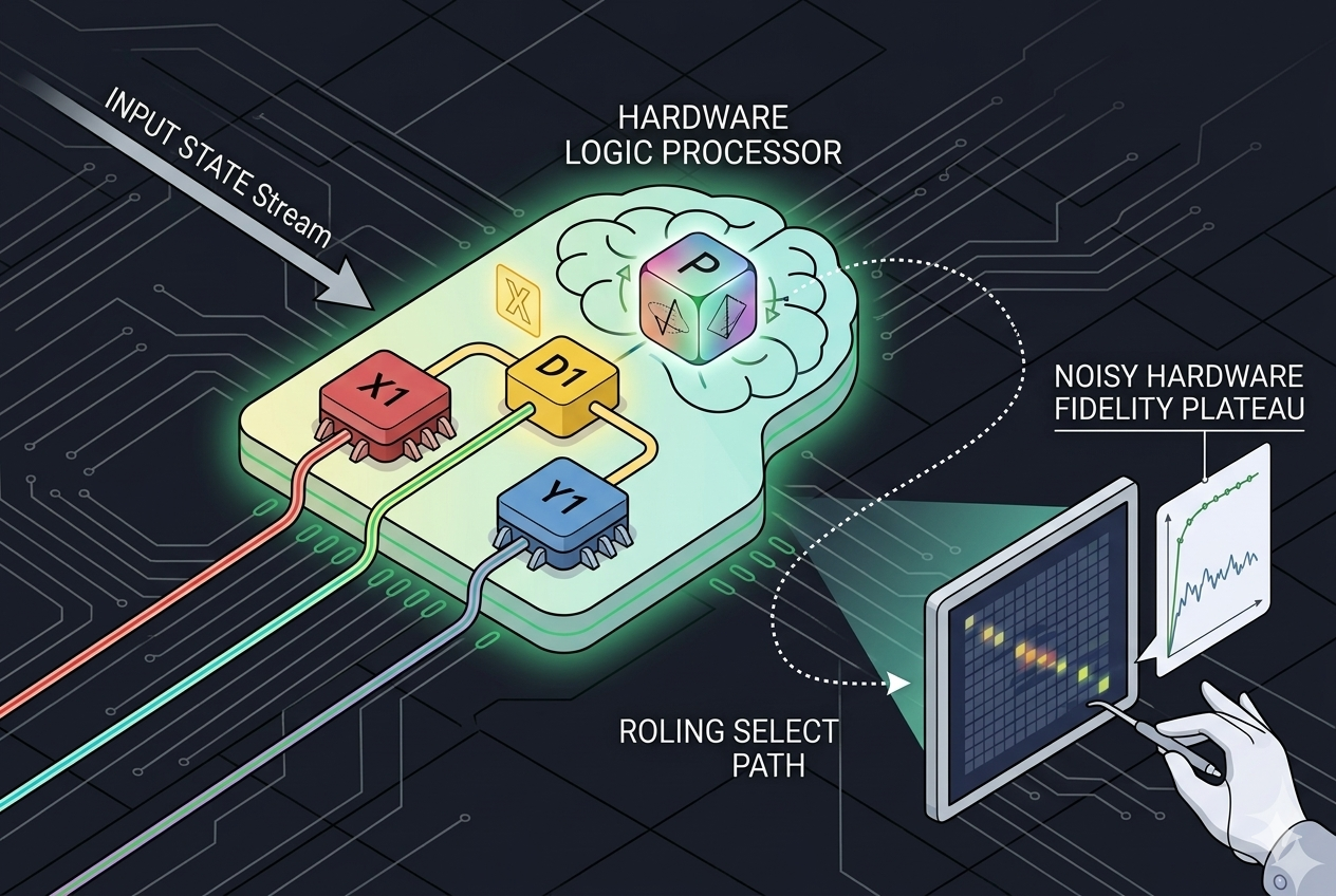
The key idea is to use a mid-circuit measurement to collapse a set of ancilla qubits into a random basis choice, which is then used to control the measurement basis of the data qubits. This allows us to effectively implement a random measurement process natively on the chip, without waiting for a classical compiler.

The protocol operates in six steps:

Prepare the data qubits in the state of interest.
Initialize a set of ancilla qubits in a superposition state that encodes the desired probability distribution over the measurement bases.
Measure the ancillas mid-circuit, collapsing them into a specific basis choice.
Feed-forward the measurement outcome to control the application of single-qubit rotations on the data qubits, physically altering the measurement basis for that specific shot.
Readout the data qubits in the standard computational basis.
Reconstruct the classical shadow by feeding the collected data into a classical algorithm to estimate the quantum state.

The Hardware Gadget

The core of this protocol relies on a specific “gadget”: one data qubit paired with two dedicated ancilla qubits. If our data qubits are kept in a line, this amounts to a tri-linear connectivity pattern where each data qubit is directly connected to two ancillas. As a proof of principle, we concentrate on a 3-qubit cluster state, which requires 3 data qubits and 6 ancillas in total.

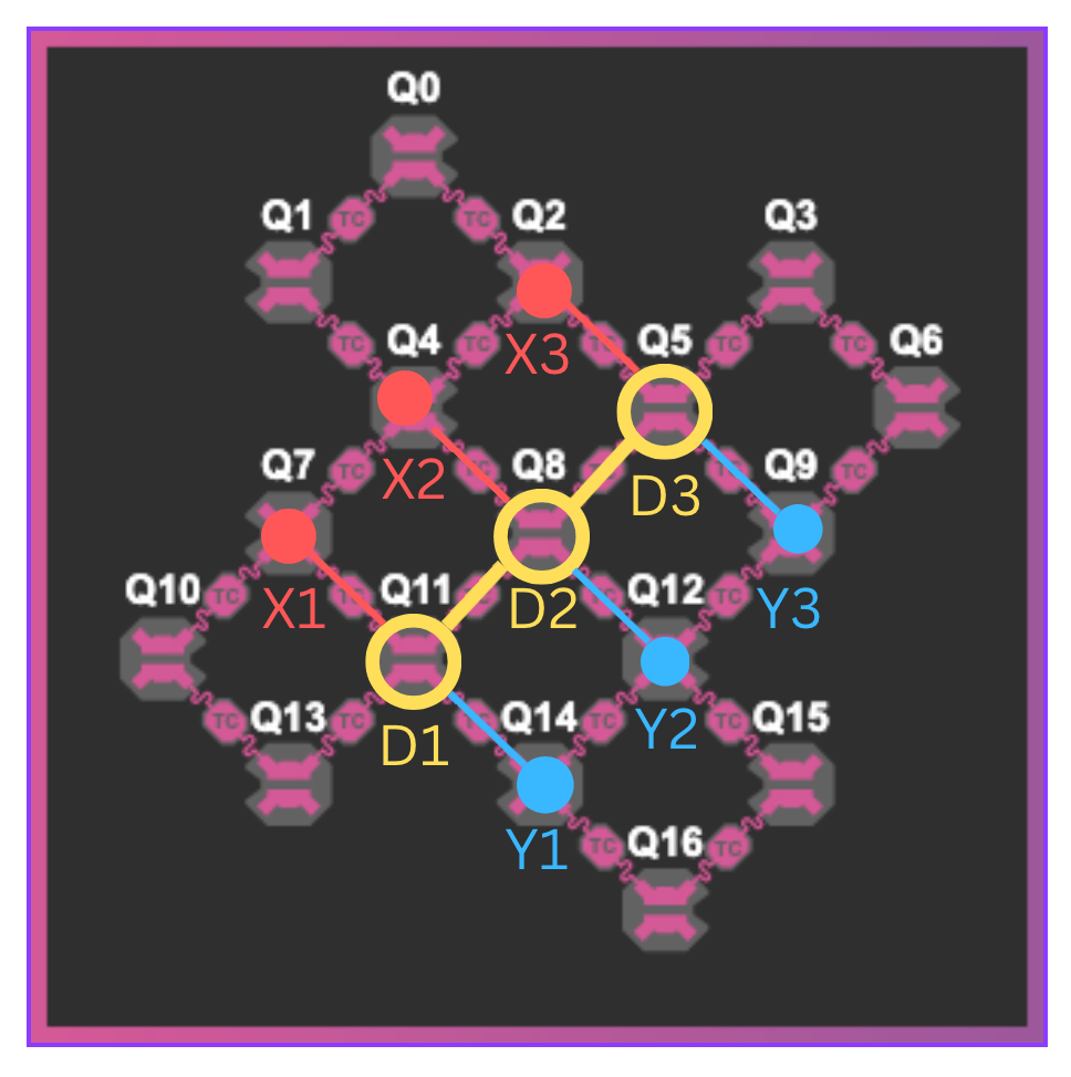
**Hardware Topology:** A 3-qubit cluster state implementation mapped onto the chip. The central data qubits (yellow, D1–D3) are each coupled to two dedicated “dice” ancilla qubits—one for controlling the X-basis (red, X1–X3) and one for the Y-basis (blue, Y1–Y3)—forming the required tri-linear connectivity pattern.

The two ancillas act as our classical dice. One ancilla controls the X vs. Z basis choice via a controlled-R_y(-\pi/2) rotation. The second ancilla controls the Y vs. Z basis choice via a controlled-R_x(\pi/2) rotation.

If we initialize the ancillas in the |+> state, they yield a uniform distribution over the outcomes. Because the controlled rotations apply based on these outcomes, the data qubit’s measurement basis maps out as follows.

00 – Z basis (no rotation), 25% probability.
10 – X basis (via Ry(-\pi/2)), 25% probability.
01 – Y basis (via Rx(\pi/2)), 25% probability.
11 – Y basis (via Ry(-\pi/2) followed by R_x(\pi/2)), 25% probability.

Notice a slight collision? Due to the non-commuting nature of the rotations, the 11 outcome also results in a Y-basis measurement. This means a naive |+> initialization actually measures Y 50% of the time!

To account for this, we can easily correct the bias by adjusting the initial rotation angles of the ancillas. We map our desired target probabilities px, py, pz into precise physical rotation angles theta1 and theta2:

def softmax_to_angles(px: float, py: float, pz: float) -> Tuple[float, float]:
    p2 = py 
    p1 = px / (px + pz + 1e-12)   

    theta1 = 2.0 * np.arcsin(np.sqrt(np.clip(p1, 0, 1)))
    theta2 = 2.0 * np.arcsin(np.sqrt(np.clip(p2, 0, 1)))
    return theta1, theta2

We then apply these angles to the ancillas during the initialization step:

for i, dq in enumerate(DATA_QUBITS):
        a1, a2 = ANCILLA_MAP[dq]
        if theta1_per_qubit[i] != 0:
            qc.ry(theta1_per_qubit[i], a1)
        if theta2_per_qubit[i] != 0:
            qc.ry(theta2_per_qubit[i], a2)
    qc.barrier()

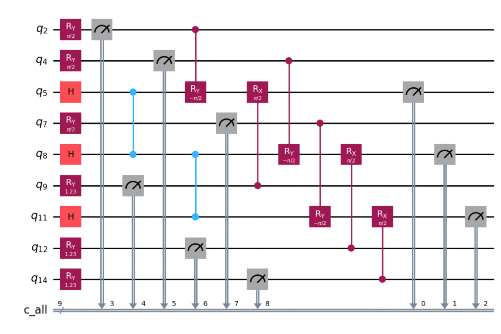
As showed in the circuit below, to get a uniform distribution px = py = pz = 1/3, we need theta1 and theta2 ~ 70.5 deg.

**The “Hardware Softmax” Circuit:** The physical circuit implementation of the on-chip logic protocol. A 3-qubit cluster state is prepared on the central data qubits (q_5, q_8, q_{11}). The six dedicated ancilla qubits are initialized with specific rotation angles (e.g., 1.23 rad ~ 70.5 deg) to encode the desired uniform measurement distribution. Mid-circuit measurements on these ancillas are then used to dynamically control the R_y(-\pi/2) and R_x(\pi/2) basis-change operations on the data qubits, natively executing the randomized shadow sampling right before the final readout.

Results

To validate the protocol, I ran this shadow tomography procedure on Quantum Inspire to characterize a 3-qubit cluster state, which has three stabilizers K_i|psi> = c_i|psi>. As you can see in the density matrix heatmaps below, qualitatively, the reconstructed density matrix matches the ideal state, proving that the mid-circuit logic executes the randomized measurements.

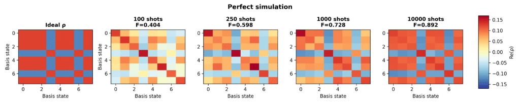
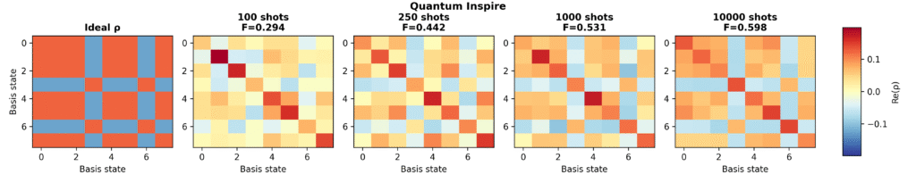
**Ideal Simulation:** Real parts of the reconstructed density matrices from a perfect, noise-free simulation of the hardware-logic protocol. As the shot count scales, the reconstructed matrix rapidly and accurately converges to the ideal 3-qubit cluster state.

**Hardware Reconstruction:** Real parts of the density matrices reconstructed natively on the Quantum Inspire hardware. While the structural footprint qualitatively matches the ideal state perfectly, hardware noise heavily dampens the amplitudes of the off-diagonal elements.

However, the reduced amplitudes of the off-diagonal density matrix elements suggest the presence of imperfections, which are most likely dominated by the limited fidelity of the gates and mid-circuit measurements on the hardware.

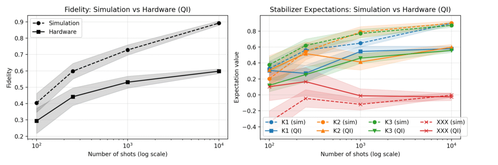
This is confirmed when we look at the fidelity between the target state and the reconstructed one, as well as the reconstructed stabilizer expectation values, which are all significantly reduced from the ideal value of 1. For comparison, we also plotted an observable that is expected to be zero.

**Convergence Metrics:** *(Left)* State fidelity scaling with the number of shots. *(Right)* Convergence of the reconstructed stabilizer expectation values (K_1, K_2, K_3) and a baseline observable expected to be zero (XXX). The gap between the simulation (dashed lines) and hardware (solid lines) highlights the plateauing effect caused by gate and mid-circuit measurement infidelities on physical chips.

Next steps

While this demonstration utilized a uniform distribution over the three Pauli bases, the true power of this “Hardware Logic” lies in its tunability. In particular, I am planning to use the protocol to implement a more active learning-based shadow tomography, where the measurement distribution is adaptively updated based on the data collected in previous shots. While it cannot achieve the same level of universality as the original classical shadow protocol, I believe it can be significantly more powerful in the presence of noisy, biased, and limited data—which is the reality of near-term quantum hardware.