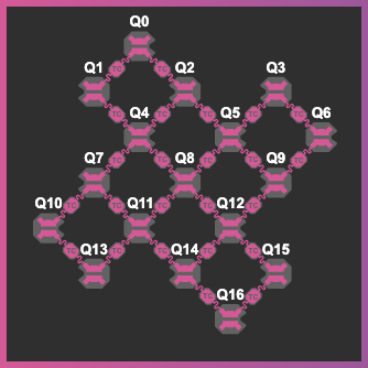
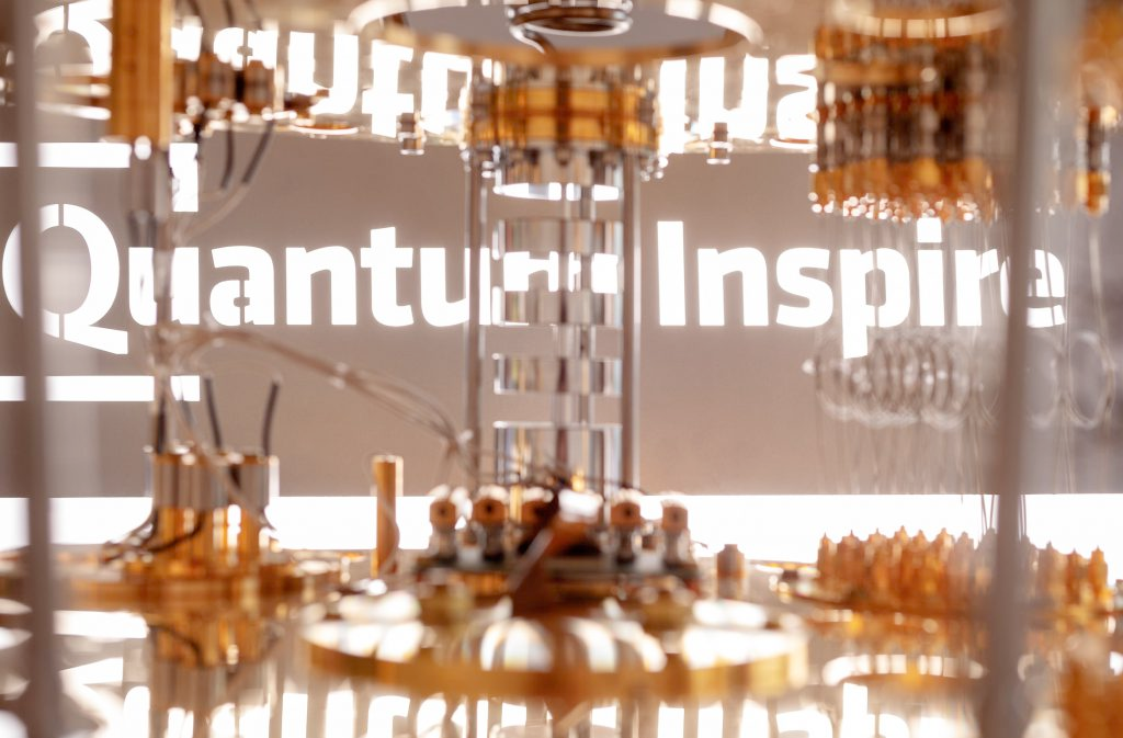
I recently got my hands on a 17-qubit superconducting transmon device of Quantum Inspire (https://www.quantum-inspire.com/).
Before developing complex quantum algorithms, I wanted to build a systems-level understanding of the hardware. In particular, I wanted to understand the role of time and space in the noise, and how the qubits interact with each other as one complex system.
Initially, I explored standard quantum benchmarks and system identification methods, but neither approach provided the right level of insight. Metrics like T1, T2, Randomized Benchmarking (RB), and Gate Set Tomography (GST) provide detailed information on individual qubits and gates, but they often treat these components in isolation. Conversely, global benchmarks like Quantum Volume or CLOPS are time-averaged, boiling performance down to a few numbers. This abstraction can obscure the underlying physics and make it difficult to diagnose specific bottlenecks.
I was looking for a “middle ground”. a model that is both interpretable and holistic, capturing how these subsystems (qubits) actually behave and interact as a cohesive whole. In the long term, an effective model that accurately captures the system’s response can be used to train control policies and develop new, noise-resilient algorithms (akin to the concept of world models []).
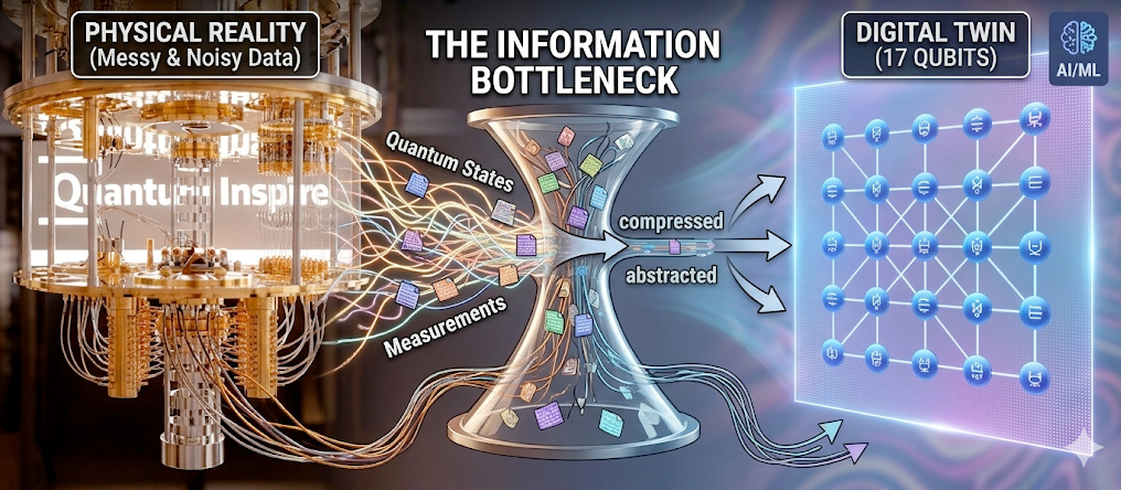
Therefore, instead of relying on traditional physical modeling, I turned to unsupervised machine learning. Using a 1D Convolutional Variational Autoencoder (Conv-VAE), I constructed a data-driven, low-dimensional representation of a noisy 17-qubit processor, serving as a digital twin to generate artificial data.
Here is how I bypassed the standard formulas and let the data describe the hardware itself.
1. The Probing Circuit (Catching the Hardware in the Act)
Revised Text
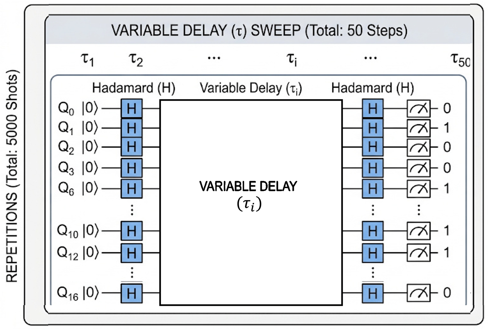
To build a digital twin, I first needed a system fingerprint, a rich dataset mapping the chip across space and time. For starters, I decided to investigate the dephasing processes, which typically limit the achievable length of quantum circuits. I went with a simple probing circuit: H−delay(τ)−H applied simultaneously across all qubits for different waiting times τ. In the absence of noise, it should always return 0, but in reality, it did not.
I designed this sequence to be sensitive to both T1 and T2* decay, as well as qubit-to-qubit correlations and spatiotemporal drift. To capture the latter, I swept the delay τ from 0.1 µs to 10 µs. This yields a single snapshot of the hardware’s behavior across all qubits. Next, this snapshot was repeated 5,000 times to observe exactly how the hardware slowly drifts. The probing sequence looks like this:
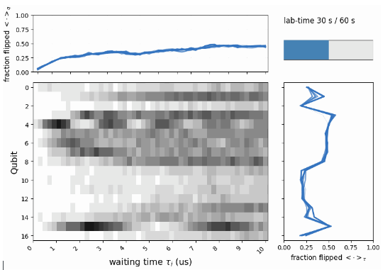
2. The raw hardware fingerprint
The result of this experiment is a massive dataset of binary 0s and 1s. When visualized, it looks like a shifting, noisy “zebra plot.”
Clearly, the qubits have their own personalities. If you look closely, you can see that this behavior is not static—there are periods where the qubits are noticeably more or less noisy (see the right plot, which averages over the waiting times, τi). This means that any model relying on a standard master equation is bound to fail, as it inherently assumes the noise is stationary and uncorrelated. The data tells a very different story.
3. The information bottleneck
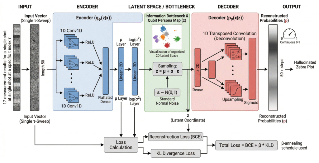
This temporal zebra plot served as the input to a data compression machine: the Variational Autoencoder (VAE). In particular, I used a convolutional version, which is capable of capturing correlations across different waiting times. I defined a single data point as a full sweep over τ for a specific qubit and repetition. System-wide correlations should therefore manifest as the collective motion of these points within the latent space.
Because the network is forced to push the data through this tiny bottleneck, it cannot simply memorize the random quantum static. Instead, it is forced to learn the underlying, interpretable physics of the system. This latent dimension parameterizes the probability distributions from which we can later draw new samples. During training, the model optimizes by minimizing the difference between the reconstructed output and the original input data.
4. Qubit personalities in the latent space
Even using an off-the-shelf architecture without any hyperparameter tuning, the distinct personalities of the qubits are already clearly visible. Below, I have plotted the latent representation for all repetitions (left) alongside the average across these repetitions (right)
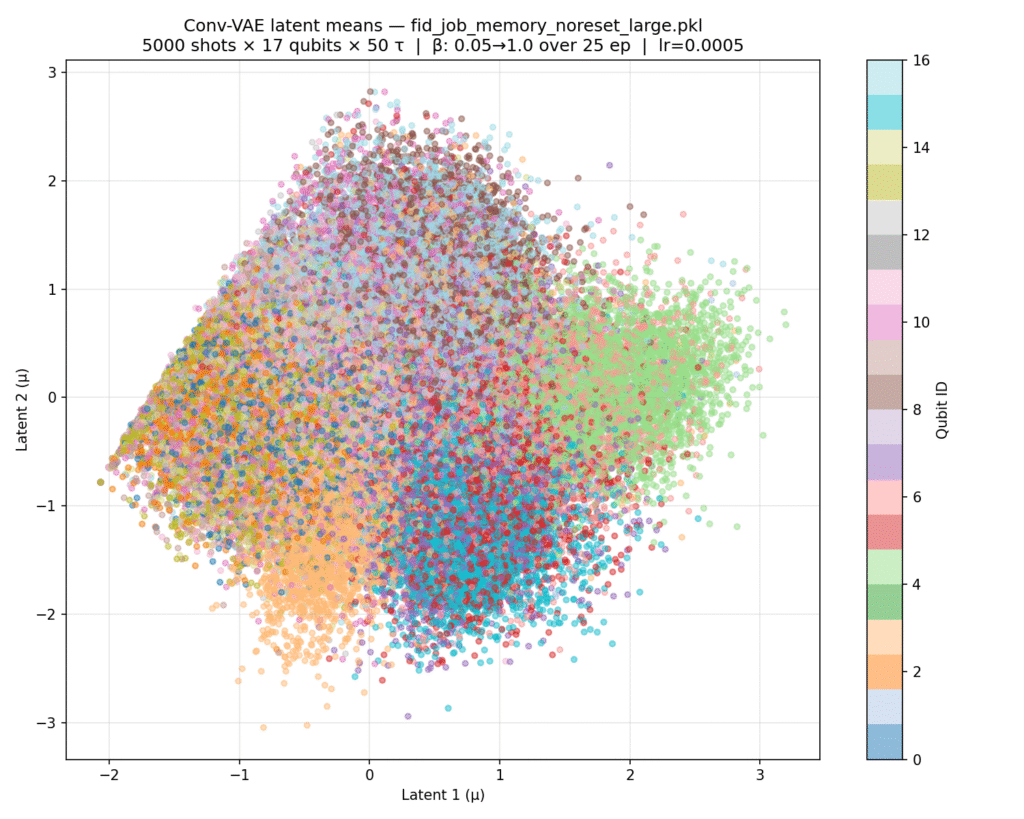
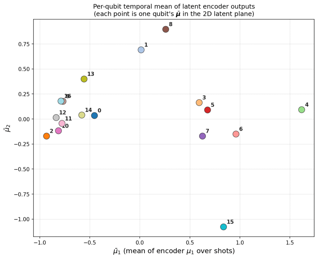
By examining the latent space, we can categorize the qubits into three distinct families:
- The Bulk: Qubits Q0, Q2, Q9, Q10–14, and Q16 are clearly clustered together. When looking at the data (averaged over 100 repetitions), we see these qubits have relatively low error rates (long coherence times) and do not exhibit any significant oscillations.
- Oscillating Qubits: There is a distinct family of qubits to the “east” of the latent plot (Q3–7) that show clear oscillations in their flip probabilities. This behavior could be attributed to miscalibration or coherent coupling to Two-Level Systems (TLS), with Q4 representing the most extreme case.
- Outliers: Finally, there are outliers situated at the opposite ends of the spectrum along the u2 axis (the second latent variable). Along this dimension, the behavior of Q15 is drastically different from Q8 and Q1. While the bulk is centered along u2, Q1 and Q8 show no oscillations but have low coherence times. Conversely, Q15 exhibits oscillations but maintains a relatively long coherence time.
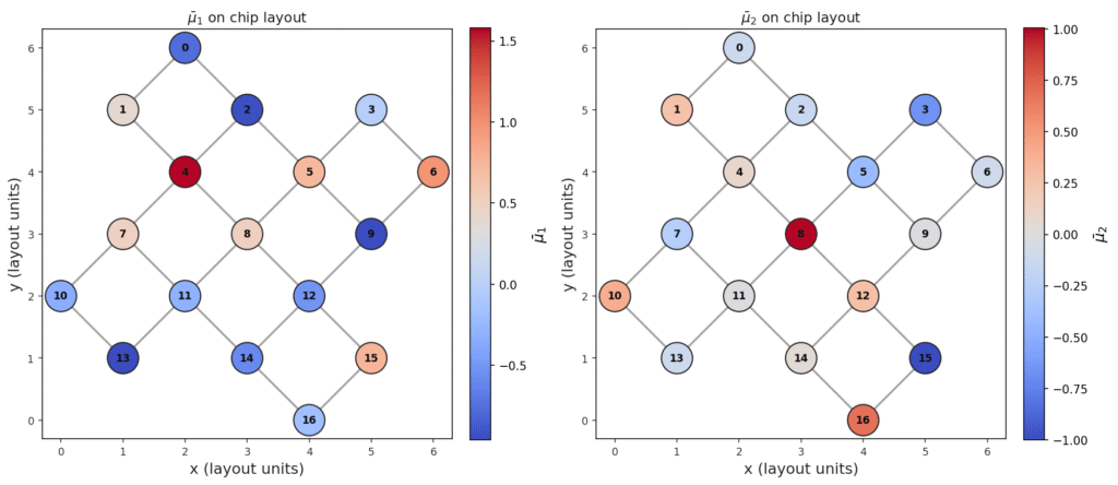
From these observations, we can interpret the physical meaning of the latent dimensions as follows:
- u1 (Coherence/Frequency): This dimension likely represents the timing of the first peak, which correlates to the coherence time or oscillation frequency (e.g., comparing the stable Q2 against the oscillating Q4).
- u2 (Decay vs. Oscillation): This dimension represents the balance between flips on the left and right sides of the sweep, effectively distinguishing between purely decaying behavior and oscillating behavior (e.g., comparing Q13 vs. Q14 or Q8 vs. Q15)
5. Tracking the Drift
Beyond static personalities, how does drift correlate across the device? Specifically, we expect qubits to shift their behavior in response to environmental events—such as the emergence of a two-level system (TLS), large-scale thermal fluctuations, or even cosmic ray impacts. To investigate this, let’s look at the trajectories in the latent space.
While most qubits exhibit a standard random walk around their mean, Q1 and Q3 show clear signs of rare, abrupt events—Lévy jumps—that temporarily alter their behavior. In particular, qubit Q3 moves from the negative u2 region all the way to the positive u2 region, briefly visiting the territory occupied by Q8. Looking back at the data in Fig. 1, this represents a transition from initially oscillating behavior to a purely decaying curve. Similarly, Q1 jumps back and forth between the “bulk” behavior and the noisy, decaying neighborhood of Q8.
This illustrates that for these qubits, coherence time is not a constant; it can temporarily plummet to match the performance of the system’s noisiest components.
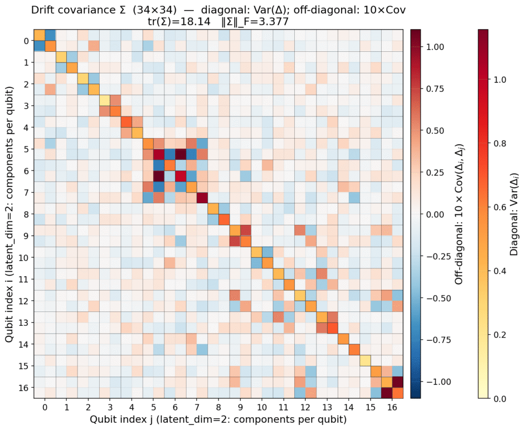
Can we use this data to extract the correlations in the drift experienced by the qubits? Specifically, do some qubits share a common origin for their drift? To answer this, we fit a simple stochastic process, an Autoregressive model of order 1 (AR(1)), to each trajectory. The extracted parameters, particularly the covariance of the random jumps, are plotted below. We also use these parameters to simulate artificial evolution within the latent space, providing a generative look at how the system’s noise profile evolves over time.
6. Generating and verifying artificial data.
With the artificial latent dynamics generated, we can now use the VAE decoder to sample entirely new, synthetic data. The result is shown in the second figure of this post. Notably, the absence of rare “Lévy jumps” in the simulated latent space makes these generated dynamics appear more stationary than the actual hardware.
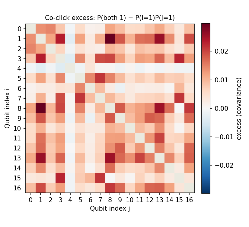
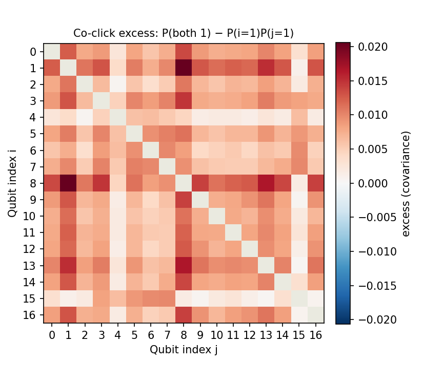
But how faithful is this reconstruction? To evaluate the model’s accuracy, we can examine spatiotemporal correlations—specifically by probing the excess of co-flips. This metric is defined as the empirically observed probability of multiple qubits flipping at the same repetition and waiting time τ, normalized by the product of their independent flipping probabilities. In essence, it tells us if the model has captured the collective “pulse” of the system rather than just the behavior of individual qubits.
7. Case study: Fast Noise
One could postulate that the VAE learned to distinguish qubits based on quasi-static modifications of the Hamiltonian—essentially identifying them by their unique drift or slow-noise signatures. To verify this hypothesis, we gathered similar data, but inserted an X pulse in the middle of the waiting time to perform a Hahn Echo sequence.
Without retraining the VAE, we analyzed the resulting latent representations. As expected, the qubits were now attracted toward the “bulk” cluster. This implies that our network interprets dynamically decoupled qubits as being nearly identical to one another; by suppressing the slow noise, we removed the very features the VAE was using to tell the qubits apart.
The only visible difference can be observed for the Q1 and Q4, which are turn out to have relatively lowest T2 time. Note also, how Q2 moves into the bulk from the outside.
Notably, retraining the network specifically on this Echo data would likely reveal a completely new representation, perhaps one based on higher-frequency noise components that the echo pulse cannot filter out.
8. Outlook
While this blog post serves as a proof-of-principle, it opens a fascinating avenue for building and controlling quantum systems within an interpretable latent space. Moving forward, one could leverage this representation to:
- Understand Hardware Operations: Observe the impact of specific gates (U) or measurements as measurable shifts in the latent space.
- Visualize Algorithms: Represent the execution of an algorithm as a trajectory through latent space, potentially aiding the discovery of new, noise-resilient protocols.
- Perform Hardware Denoising: Use the VAE’s bottleneck to filter out “quantum static” and improve the fidelity of the system’s output.
- Scalable Benchmarking: Compare the latent signatures of different quantum processors in a standardized, scalable way.
- Real-time Diagnostics: Identify miscalibrated qubits and detect rare “black swan” events (such as jumps or TLS fluctuations) as they occur.
- RL & World Models: Use the generative capabilities of this digital twin to train Reinforcement Learning (RL) agents to stabilize and control the device in real-time.
That is just the beginning. The goal is to move beyond mere observation and into a regime where we can navigate the noise of a quantum processor as easily as we navigate a map.
Share: